Everything you need to know about TensorFlow 2.0
On June 26 of 2019, I will be giving a TensorFlow (TF) 2.0 workshop at the PAPIs.io LATAM conference in São Paulo. Aside from the happiness of being representing Daitan as the workshop host, I am very happy to talk about TF 2.0.
The idea of the workshop is to highlight what has changed from the previous 1.x version of TF. In this text, you can follow along with the main topics we are going to discuss. And of course, have a look at the Colab notebook for practical code.
Introduction to TensorFlow 2.0
TensorFlow is a general purpose high-performance computing library open sourced by Google in 2015. Since the beginning, its main focus was to provide high-performance APIs for building Neural Networks (NNs). However, with the advance of time and interest by the Machine Learning (ML) community, the lib has grown to a full ML ecosystem.
Currently, the library is experiencing its largest set of changes since its birth. TensorFlow 2.0 is currently in beta and brings many changes compared to TF 1.x. Let’s dive into the main ones.
Eager Execution By Default
To start, eager execution is the default way of running TF code.
As you might recall, to build a Neural Net in TF 1.x, we needed to define this abstract data structure called a Graph. Also, (as you probably have tried), if we attempted to print one of the graph nodes, we would not see the values we were expecting. Instead, we would see a reference to the graph node. To actually, run the graph, we needed to use an encapsulation called a Session. And using the Session.run() method, we could pass Python data to the graph and actually train our models.
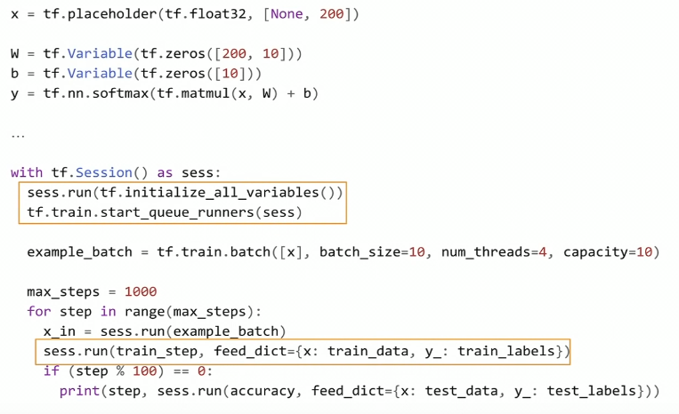
With eager execution, this changes. Now, TensorFlow code can be run like normal Python code. Eagerly. Meaning that operations are created and evaluated at once.
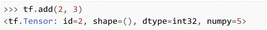
TensorFlow 2.0 code looks a lot like NumPy code. In fact, TensorFlow and NumPy objects can easily be switched from one to the other. Hence, you do not need to worry about placeholders, Sessions, feed_dictionaties, etc.
API Cleanup
Many APIs like tf.gans, tf.app, tf.contrib, tf.flags are either gone or moved to separate repositories.
However, one of the most important cleanups relates to how we build models. You may remember that in TF 1.x we have many more than 1 or 2 different ways of building/training ML models.
Tf.slim, tf.layers, tf.contrib.layers, tf.keras are all possible APIs one can use to build NNs is TF 1.x. That not to include the Sequence to Sequence APIs in TF 1.x. And most of the time, it was not clear which one to choose for each situation.
Although many of these APIs have great features, they did not seem to converge to a common way of development. Moreover, if we trained a model in one of these APIs, it was not straight forward to reuse that code using the other ones.
In TF 2.0, tf.keras is the recommended high-level API.
As we will see, Keras API tries to address all possible use cases.
The Beginners API
From TF 1.x to 2.0, the beginner API did not change much. But now, Keras is the default and recommended high-level API. In summary, Keras is a set of layers that describes how to build neural networks using a clear standard. Basically, when we install TensorFlow using pip, we get the full Keras API plus some additional functionalities.
model = tf.keras.models.Sequential()
model.add(Flatten(input_shape=(IMAGE_HEIGHT,IMAGE_WIDTH)))
model.add(Dense(units=32, activation='relu'))
model.add(Dropout(0.3))
model.add(Dense(units=32, activation='relu'))
model.add(Dense(units=10, activation='softmax'))

# Configures the model for training.
# Define the model optimizer, the loss function and the accuracy metrics
model.compile(optimizer='adam',
              loss='sparse_categorical_crossentropy',
              metrics=['accuracy'])
model.summary()
The beginner’s API is called Sequential. It basically defines a neural network as a stack of layers. Besides its simplicity, it has some advantages. Note that we define our model in terms of a data structure (a stack of layers). As a result, it minimizes the probability of making errors due to model definition.
Keras-Tuner
Keras-tuner is a dedicated library for hyper-parameter tuning of Keras models. As of this writing, the lib is in pre-alpha status but works fine on Colab with tf.keras and Tensorflow 2.0 beta.
It is a very simple concept. First, need to define a model building function that returns a compiled keras model. The function takes as input a parameter called hp. Using hp, we can define a range of candidate values that we can sample hyper-parameters values.
Below we build a simple model and optimize over 3 hyper-parameters. For the hidden units, we sample integer values between a pre-defined range. For dropout and learning rate, we choose at random, between some specified values.
def build_model(hp):
  # define the hyper parameter ranges for the learning rate, dropout and hidden unit
  hp_units = hp.Range('units', min_value=32, max_value=128, step=32)
  hp_lr = hp.Choice('learning_rate', values=[1e-2, 1e-3, 1e-4])
  hp_dropout = hp.Choice('dropout', values=[0.1,0.2,0.3])

  # build a Sequential model
  model = keras.Sequential()
  model.add(Flatten(input_shape=(IMAGE_HEIGHT,IMAGE_WIDTH)))
  model.add(Dense(units=hp_units, activation='relu'))
  model.add(Dropout(hp_dropout))
  model.add(Dense(units=32, activation='relu'))
  model.add(layers.Dense(10, activation='softmax'))

  # compile and return the model
  model.compile(optimizer=keras.optimizers.Adam(hp_lr),
      loss='sparse_categorical_crossentropy',
      metrics=['accuracy'])
  return model

# create a Random Search tuner
tuner = RandomSearch(
    build_model,
    objective='val_accuracy', # define the metric to be optimized over
    max_trials=3,
    executions_per_trial=1,
    directory='my_logs') # define the output log/checkpoints folder

 # start hyper-parameter optmization search
tuner.search(x_train, y_train,
             epochs=2,
             validation_data=(x_test, y_test))
Then, we create a tuner object. In this case, it implements a Random Search Policy. Lastly, we can start optimization using the search() method. It has the same signature as fit().
In the end, we can check the tuner summary results and choose the best model(s). Note that training logs and model checkpoints are all saved in the directory folder (my_logs). Also, the choice of minimizing or maximizing the objective (validation accuracy) is automatically infered.
Have a look at their Github page to learn more.
The Advanced API
The moment you see this type of implementation it goes back to Object Oriented programming. Here, your model is a Python class that extends tf.keras.Model. Model subclassing is an idea inspired by Chainer and relates very much to how PyTorch defines models.
With model Subclassing, we define the model layers in the class constructor. And the call() method handles the definition and execution of the forward pass.
class Model(tf.keras.Model):
  def __init__(self):
    # Define the layers here
    super(Model, self).__init__()
    self.conv1 = Conv2D(filters=8, kernel_size=4, padding="same", strides=1, input_shape=(IMAGE_HEIGHT,IMAGE_WIDTH,IMAGE_DEPTH))
    self.conv2 = Conv2D(filters=16, kernel_size=4, padding="same", strides=1)
    self.pool = MaxPool2D(pool_size=2, strides=2, padding="same")
    self.flat = Flatten()
    self.probs = Dense(units=N_CLASSES, activation='softmax', name="output")

  def call(self, x):
    # Define the forward pass
    net = self.conv1(x)
    net = self.pool(net)
    net = self.conv2(net)
    net = self.pool(net)
    net = self.flat(net)
    net = self.probs(net)
    return net

  def compute_output_shape(self, input_shape):
    # You need to override this function if you want to use the subclassed model
    # as part of a functional-style model.
    # Otherwise, this method is optional.
    shape = tf.TensorShape(input_shape).as_list()
    shape[-1] = self.num_classes
    return tf.TensorShape(shape)
subclassing_model.py
Subclassing has many advantages. It is easier to perform a model inspection. We can, (using breakpoint debugging), stop at a given line and inspect the model’s activations or logits.
However, with great flexibility comes more bugs.
Model Subclassing requires more attention and knowledge from the programmer.
In general, your code is more prominent to errors (like model wiring).
Defining the Training Loop
The easiest way to train a model in TF 2.0 is by using the fit() method. fit() supports both types of models, Sequential and Subclassing. The only adjustment you need to do, if using model Subclassing, is to override the compute_output_shape() class method, otherwise, you can through it away. Other than that, you should be able to use fit() with either tf.data.Dataset or standard NumPy nd-arrays as input.
However, if you want a clear understanding of what is going on with the gradients or the loss, you can use the Gradient Tape. That is especially useful if you are doing research.
Using Gradient Tape, one can manually define each step of a training procedure. Each of the basic steps in training a neural net such as:
- Forward pass
- Loss function evaluation
- Backward pass
- Gradient descent step
is separately specified.
This is much more intuitive if one wants to get a feel of how a Neural Net is trained. If you want to check the loss values w.r.t the model weights or the gradient vectors itself, you can just print them out.
Gradient Tape gives much more flexibility. But just like Subclassing vs Sequential, more flexibility comes with an extra cost. Compared to the fit() method, here we need to define a training loop manually. As a natural consequence, it makes the code more prominent to bugs and harder to debug. I believe that is a great trade off that works ideally for code engineers (looking for standardized code), compared to researchers who usually are interested in developing something new.
Also, using fit() we can easily setup TensorBoard as we see next.
Setting up TensorBoard
You can easily setup an instance of TensorBoard using the fit() method. It also works on Jupyter/Colab notebooks.
In this case, you add TensorBoard as a callback to the fit method.
As long as you are using the fit() method, it works on both: Sequential and the Subclassing APIs.
# Load the TensorBoard notebook extension
%load_ext tensorboard

# create the tensorboard callback
tensorboard = TensorBoard(log_dir='logs/{}'.format(time.time()), histogram_freq=1)

# train the model
model.fit(x=x_train,
          y=y_train,
          epochs=2,
          validation_data=(x_test, y_test),
          callbacks=[tensorboard])

# launch TensorBoard
%tensorboard --logdir logs
If you choose to use Model Subclassing and write the training loop yourself (using Grading Tape), you also need to define TensorBoard manually. It involves creating the summary files, using tf.summary.create_file_writer(), and specifying which variables you want to visualize.
As a worth noting point, there are many callbacks you can use. Some of the more useful ones are:
- EarlyStopping: As the name implies, it sets up a rule to stop training when a monitored quantity has stopped improving.
- ReduceLROnPlateau: Reduce the learning rate when a metric has stopped improving.
- TerminateOnNaN: Callback that terminates training when a NaN loss is encountered.
- LambdaCallback: Callback for creating simple, custom callbacks on-the-fly.
You can check the complete list at TensorFlow 2.0 callbacks.
Extracting Performance of your EagerCode
If you choose to train your model using Gradient Tape, you will notice a substantial decrease in performance.
Executing TF code eagerly is good for understanding, but it fails on performance. To avoid this problem, TF 2.0 introduces tf.function.
Basically, if you decorate a python function with tf.function, you are asking TensorFlow to take your function and convert it to a TF high-performance abstraction.
@tf.function
def train_step(images, labels):

  with tf.GradientTape() as tape:
    # forward pass
    predictions = model(images)

    # compute the loss
    loss = cross_entropy(tf.one_hot(labels, N_CLASSES), predictions)

  # get the gradients w.r.t the model's weights
  gradients = tape.gradient(loss, model.trainable_variables)

  # perform a gradient descent step
  optimizer.apply_gradients(zip(gradients, model.trainable_variables))

  # accumulates the training loss and accuracy
  train_loss(loss)
  train_accuracy(labels, predictions)
tf_function.py
It means that the function will be marked for JIT compilation so that TensorFlow runs it as a graph. As a result, you get the performance benefits of TF 1.x (graphs) such as node pruning, kernel fusion, etc.
In short, the idea of TF 2.0 is that you can devise your code into smaller functions. Then, you can annotate the ones you wish using tf.function, to get this extra performance. It is best to decorate functions that represent the largest computing bottlenecks. These are usually the training loops or the model’s forward pass.
Note that when you decorate a function with tf.function, you loose some of the benefits of eager execution. In other words, you will not be able to setup breakpoints or use print() inside that section of code.
Save and Restore Models
Another great lack of standardization in TF 1.x is how we save/load trained models for production. TF 2.0 also tries to address this problem by defining a single API.
Instead of having many ways of saving models, TF 2.0 standardize to an abstraction called the SavedModel.
There is no much to say here. If you create a Sequential model or extend your class using tf.keras.Model, your class inherits from tf.train.Checkpoints. As a result, you can serialize your model to a SavedModel object.
# serialize your model to a SavedModel object
# It includes the entire graph, all variables and weights
model.save('/tmp/model', save_format='tf')

# load your saved model
model = tf.keras.models.load_model('/tmp/model')
SavedModels are integrated with the TensorFlow ecosystem. In other words, you will be able to deploy it to many different devices. These include mobile phones, edge devices, and servers.
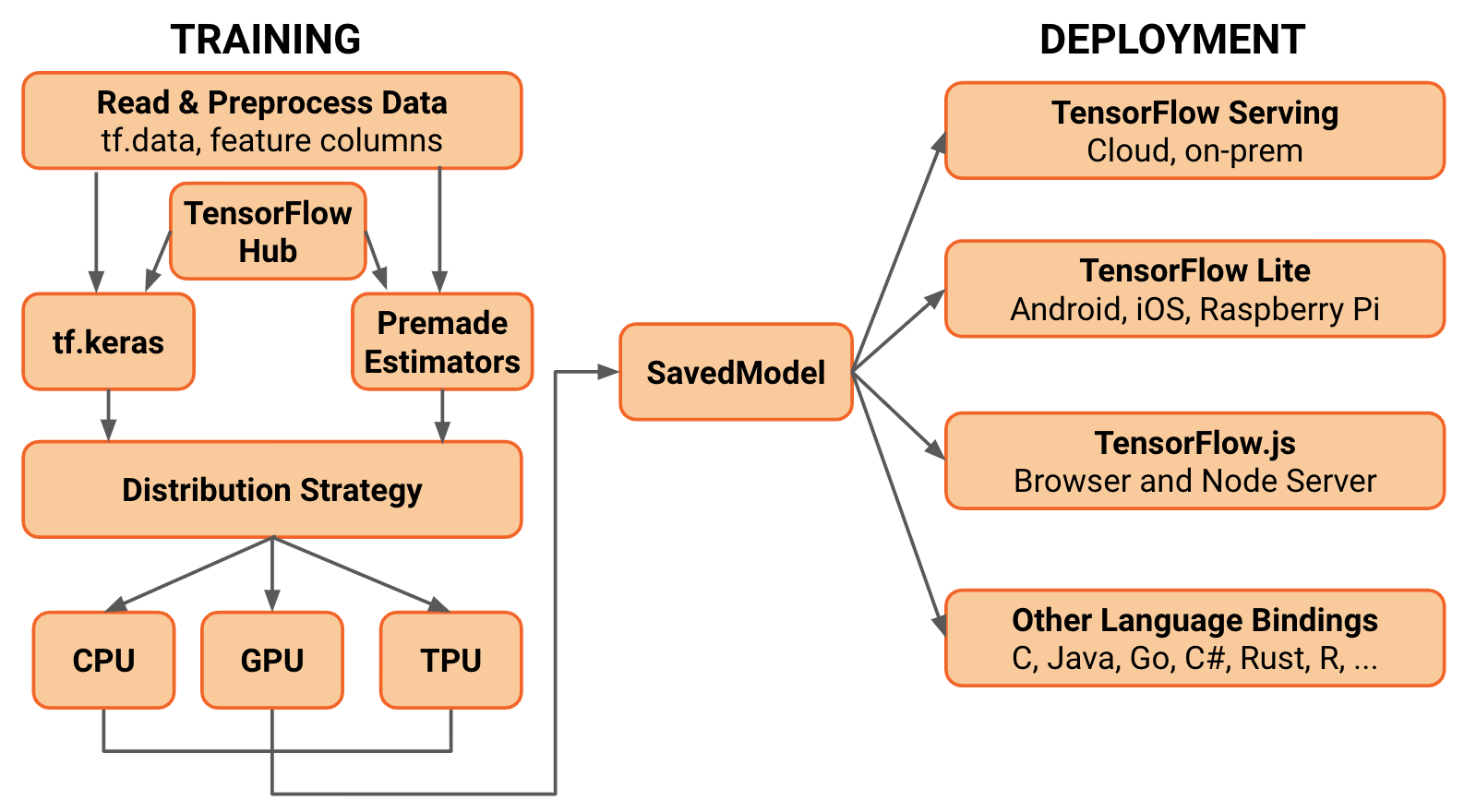
Converting to TF-Lite
If you want to deploy a SavedModel to embedded devices like Raspberry Pi, Edge TPUs or your phone, use the TF Lite converter.
Note that in 2.0, the TFLiteConverter does not support frozen GraphDefs (usually generated in TF 1.x). If you want to convert a frozen GraphDefs to run in TF 2.0, you can use the tf.compat.v1.TFLiteConverter.
It is very common to perform post-training quantization before deploying to embedded devices. To do it with the TFLiteConverter, set the optimizations flag to “OPTIMIZE_FOR_SIZE”. This will quantize the model’s weights from floating point to 8-bits of precision. It will reduce the model size and improve latency with little degradation in model accuracy.
# create a TF Lite converter
converter = tf.lite.TFLiteConverter.from_keras_model(model)

# performs model quantization to reduce the size of the model and improve latency
converter.optimizations = [tf.lite.Optimize.OPTIMIZE_FOR_SIZE]

tflite_model = converter.convert()
Note that this is an experimental flag, and it is subject to changes.
Converting to TensorFlow.js
To close up, we can also take the same SavedModel object and convert it to TensorFlow.js format. Then, we can load it using Javascript and run your model on the Browser.
!tensorflowjs_converter \
    --input_format=tf_saved_model \
    --saved_model_tags=serve \
    --output_format=tfjs_graph_model \
    /tmp/model \
    /tmp/web_model
tensorflowjs_converter.sh
First, you need to install TensorFlow.js via pip. Then, use the tensorflowjs_converter script to take your trained-model and convert to Javascript compatible code. Finally, you can load it and perform inference in Javascript.
You can also train models using Tesnorflow.js on the Browser.
Conclusions
To close off, I would like to mention some other capabilities of 2.0. First, we have seen that adding more layers to a Sequential or Subclassing model is very straightforward. And, although TF covers most of the popular layers like Conv2D, TransposeConv2D etc; you can always find yourself in a situation where you need something that is not available. That is especially true if you are reproducing some paper or doing research.
The good news is that we can develop our own Custom layers. Following the same Keras API, we can create a class and extend it to tf.keras.Layer. In fact, we can create custom activation functions, regularization layers, or metrics following a very similar pattern. Here is a good resource about it.
Also, we can convert existing TensorFlow 1.x code to TF 2.0. For this end, the TF team created the tf_upgrade_v2 utility.
This script does not convert TF 1.x code to 2.0 idiomatics. It basically uses tf.compat.v1 module for functions that got their namespaces changed. Also, if your legacy code uses tf.contrib, the script will not be able to convert it. You will probably need to use additional libraries or use the new TF 2.0 version of the missing functions.
Thanks for reading.
☞ Understand TensorFlow by mimicking its API from scratchTheory
☞ How to get started with Machine Learning in about 10 minutes
☞ Introduction to Multilayer Neural Networks with TensorFlow’s Keras API
☞ TensorFlow.js Crash Course – Machine Learning For The Web – Getting Started
Suggest:
☞ Machine Learning Zero to Hero - Learn Machine Learning from scratch
☞ Complete Python Tutorial for Beginners (2019)
☞ Python Tutorials for Beginners - Learn Python Online
☞ What is Python and Why You Must Learn It in [2019]