Recurrent Neural Networks by Example in Python

Recurrent Neural Network

It’s helpful to understand at least some of the basics before getting to the implementation. At a high level, a recurrent neural network (RNN) processes sequences — whether daily stock prices, sentences, or sensor measurements — one element at a time while retaining a memory (called a state) of what has come previously in the sequence.

Recurrent means the output at the current time step becomes the input to the next time step. At each element of the sequence, the model considers not just the current input, but what it remembers about the preceding elements.

This memory allows the network to learn long-term dependencies in a sequence which means it can take the entire context into account when making a prediction, whether that be the next word in a sentence, a sentiment classification, or the next temperature measurement. A RNN is designed to mimic the human way of processing sequences: we consider the entire sentence when forming a response instead of words by themselves. For example, consider the following sentence:

“The concert was boring for the first 15 minutes while the band warmed up but then was terribly exciting.”

A machine learning model that considers the words in isolation — such as a bag of words model — would probably conclude this sentence is negative. An RNN by contrast should be able to see the words “but” and “terribly exciting” and realize that the sentence turns from negative to positive because it has looked at the entire sequence. Reading a whole sequence gives us a context for processing its meaning, a concept encoded in recurrent neural networks.

At the heart of an RNN is a layer made of memory cells. The most popular cell at the moment is the Long Short-Term Memory (LSTM) which maintains a cell state as well as a carry for ensuring that the signal (information in the form of a gradient) is not lost as the sequence is processed. At each time step the LSTM considers the current word, the carry, and the cell state.

The LSTM has 3 different gates and weight vectors: there is a “forget” gate for discarding irrelevant information; an “input” gate for handling the current input, and an “output” gate for producing predictions at each time step. However, as Chollet points out, it is fruitless trying to assign specific meanings to each of the elements in the cell.

The function of each cell element is ultimately decided by the parameters (weights) which are learned during training. Feel free to label each cell part, but it’s not necessary for effective use! Recall, the benefit of a Recurrent Neural Network for sequence learning is it maintains a memory of the entire sequence preventing prior information from being lost.

Problem Formulation

There are several ways we can formulate the task of training an RNN to write text, in this case patent abstracts. However, we will choose to train it as a many-to-one sequence mapper. That is, we input a sequence of words and train the model to predict the very next word. The words will be mapped to integers and then to vectors using an embedding matrix (either pre-trained or trainable) before being passed into an LSTM layer.

When we go to write a new patent, we pass in a starting sequence of words, make a prediction for the next word, update the input sequence, make another prediction, add the word to the sequence and continue for however many words we want to generate.

The steps of the approach are outlined below:

1. Convert abstracts from list of strings into list of lists of integers (sequences)
2. Create feature and labels from sequences
3. Build LSTM model with Embedding, LSTM, and Dense layers
4. Load in pre-trained embeddings
5. Train model to predict next work in sequence
6. Make predictions by passing in starting sequence

Keep in mind this is only one formulation of the problem: we could also use a character level model or make predictions for each word in the sequence. As with many concepts in machine learning, there is no one correct answer, but this approach works well in practice.

Data Preparation

Even with a neural network’s powerful representation ability, getting a quality, clean dataset is paramount. The raw data for this project comes from USPTO PatentsView, where you can search for information on any patent applied for in the United States. I searched for the term “neural network” and downloaded the resulting patent abstracts — 3500 in all. I found it best to train on a narrow subject, but feel free to try with a different set of patents.

We’ll start out with the patent abstracts as a list of strings. The main data preparation steps for our model are:

1. Remove punctuation and split strings into lists of individual words
2. Convert the individual words into integers

These two steps can both be done using the Keras [Tokenizer](https://keras.io/preprocessing/text/#tokenizer) class. By default, this removes all punctuation, lowercases words, and then converts words to sequences of integers. A Tokenizer is first fit on a list of strings and then converts this list into a list of lists of integers. This is demonstrated below:

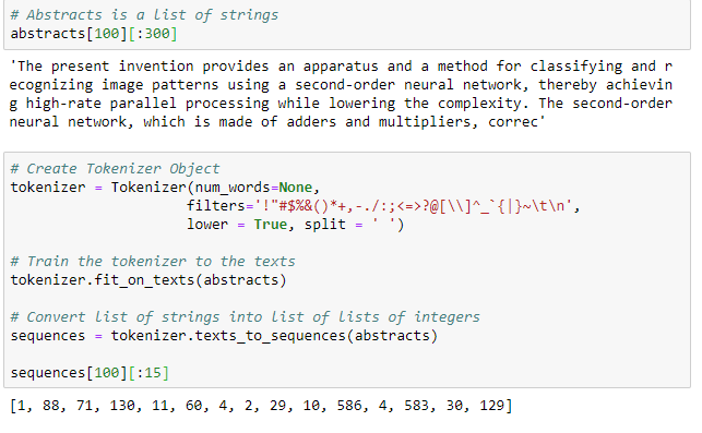
The output of the first cell shows the original abstract and the output of the second the tokenized sequence. Each abstract is now represented as integers.

We can use the idx_word attribute of the trained tokenizer to figure out what each of these integers means:

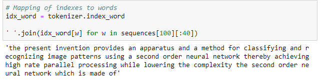
If you look closely, you’ll notice that the Tokenizer has removed all punctuation and lowercased all the words. If we use these settings, then the neural network will not learn proper English! We can adjust this by changing the filters to the Tokenizer to not remove punctuation.

# Don't remove punctuation or uppercase
tokenizer = Tokenizer(num_words=None, 
                     filters='#$%&()*+-<=>@[\\]^_`{|}~\t\n',
                     lower = False, split = ' ')

See the notebooks for different implementations, but, when we use pre-trained embeddings, we’ll have to remove the uppercase because there are no lowercase letters in the embeddings. When training our own embeddings, we don’t have to worry about this because the model will learn different representations for lower and upper case.

Features and Labels

The previous step converts all the abstracts to sequences of integers. The next step is to create a supervised machine learning problem with which to train the network. There are numerous ways you can set up a recurrent neural network task for text generation, but we’ll use the following:

Give the network a sequence of words and train it to predict the next word.

The number of words is left as a parameter; we’ll use 50 for the examples shown here which means we give our network 50 words and train it to predict the 51st. Other ways of training the network would be to have it predict the next word at each point in the sequence — make a prediction for each input word rather than once for the entire sequence — or train the model using individual characters. The implementation used here is not necessarily optimal — there is no accepted best solution —_ but it works well_!

Creating the features and labels is relatively simple and for each abstract (represented as integers) we create multiple sets of features and labels. We use the first 50 words as features with the 51st as the label, then use words 2–51 as features and predict the 52nd and so on. This gives us significantly more training data which is beneficial because the performance of the network is proportional to the amount of data that it sees during training.

The implementation of creating features and labels is below:

features = []
labels = []

training_length = 50

# Iterate through the sequences of tokens
for seq in sequences:

    # Create multiple training examples from each sequence
    for i in range(training_length, len(seq)):
        
        # Extract the features and label
        extract = seq[i - training_length:i + 1]

        # Set the features and label
        features.append(extract[:-1])
        labels.append(extract[-1])
        
features = np.array(features)

The features end up with shape (296866, 50) which means we have almost 300,000 sequences each with 50 tokens. In the language of recurrent neural networks, each sequence has 50 timesteps each with 1 feature.

We could leave the labels as integers, but a neural network is able to train most effectively when the labels are one-hot encoded. We can one-hot encode the labels with numpy very quickly using the following:

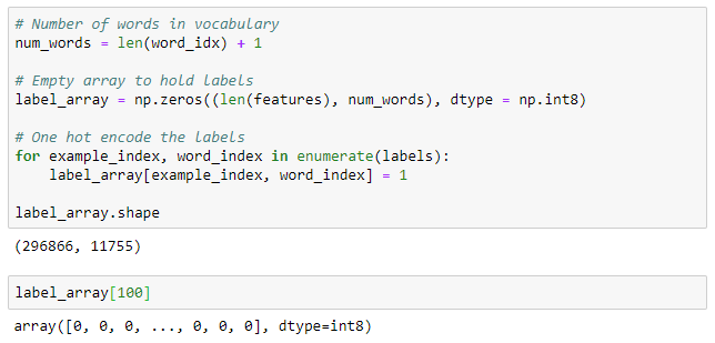
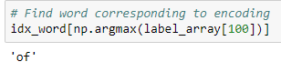
To find the word corresponding to a row in label_array , we use:

After getting all of our features and labels properly formatted, we want to split them into a training and validation set (see notebook for details). One important point here is to shuffle the features and labels simultaneously so the same abstracts do not all end up in one set.

Building a Recurrent Neural Network

Keras is an incredible library: it allows us to build state-of-the-art models in a few lines of understandable Python code. Although other neural network libraries may be faster or allow more flexibility, nothing can beat Keras for development time and ease-of-use.

The code for a simple LSTM is below with an explanation following:

from keras.models import Sequential
from keras.layers import LSTM, Dense, Dropout, Masking, Embedding

model = Sequential()

# Embedding layer
model.add(
    Embedding(input_dim=num_words,
              input_length = training_length,
              output_dim=100,
              weights=[embedding_matrix],
              trainable=False,
              mask_zero=True))

# Masking layer for pre-trained embeddings
model.add(Masking(mask_value=0.0))

# Recurrent layer
model.add(LSTM(64, return_sequences=False, 
               dropout=0.1, recurrent_dropout=0.1))

# Fully connected layer
model.add(Dense(64, activation='relu'))

# Dropout for regularization
model.add(Dropout(0.5))

# Output layer
model.add(Dense(num_words, activation='softmax'))

# Compile the model
model.compile(
    optimizer='adam', loss='categorical_crossentropy', metrics=['accuracy'])

We are using the Keras Sequential API which means we build the network up one layer at a time. The layers are as follows:

• An Embedding which maps each input word to a 100-dimensional vector. The embedding can use pre-trained weights (more in a second) which we supply in the weights parameter. trainable can be set False if we don’t want to update the embeddings.
• A Masking layer to mask any words that do not have a pre-trained embedding which will be represented as all zeros. This layer should not be used when training the embeddings.
• The heart of the network: a layer of LSTM cells with dropout to prevent overfitting. Since we are only using one LSTM layer, it does not return the sequences, for using two or more layers, make sure to return sequences.
• A fully-connected Dense layer with relu activation. This adds additional representational capacity to the network.
• A Dropout layer to prevent overfitting to the training data.
• A Dense fully-connected output layer. This produces a probability for every word in the vocab using softmax activation.

The model is compiled with the Adam optimizer (a variant on Stochastic Gradient Descent) and trained using the categorical_crossentropy loss. During training, the network will try to minimize the log loss by adjusting the trainable parameters (weights). As always, the gradients of the parameters are calculated using back-propagation and updated with the optimizer. Since we are using Keras, we don’t have to worry about how this happens behind the scenes, only about setting up the network correctly.

Without updating the embeddings, there are many fewer parameters to train in the network. The input to the [LSTM](https://machinelearningmastery.com/reshape-input-data-long-short-term-memory-networks-keras/) layer is [(None, 50, 100)](https://machinelearningmastery.com/reshape-input-data-long-short-term-memory-networks-keras/) which means that for each batch (the first dimension), each sequence has 50 timesteps (words), each of which has 100 features after embedding. Input to an LSTM layer always has the (batch_size, timesteps, features) shape.

There are many ways to structure this network and there are several others covered in the notebook. For example, we can use two LSTM layers stacked on each other, a Bidirectional LSTM layer that processes sequences from both directions, or more Dense layers. I found the set-up above to work well.

Pre-Trained Embeddings

Once the network is built, we still have to supply it with the pre-trained word embeddings. There are numerous embeddings you can find online trained on different corpuses (large bodies of text). The ones we’ll use are available from Stanford and come in 100, 200, or 300 dimensions (we’ll stick to 100). These embeddings are from the GloVe (Global Vectors for Word Representation) algorithm and were trained on Wikipedia.

Even though the pre-trained embeddings contain 400,000 words, there are some words in our vocab that are included. When we represent these words with embeddings, they will have 100-d vectors of all zeros. This problem can be overcome by training our own embeddings or by setting the Embedding layer’s trainable parameter to True (and removing the Masking layer).

We can quickly load in the pre-trained embeddings from disk and make an embedding matrix with the following code:

# Load in embeddings
glove_vectors = '/home/ubuntu/.keras/datasets/glove.6B.100d.txt'
glove = np.loadtxt(glove_vectors, dtype='str', comments=None)

# Extract the vectors and words
vectors = glove[:, 1:].astype('float')
words = glove[:, 0]

# Create lookup of words to vectors
word_lookup = {word: vector for word, vector in zip(words, vectors)}

# New matrix to hold word embeddings
embedding_matrix = np.zeros((num_words, vectors.shape[1]))

for i, word in enumerate(word_idx.keys()):
    # Look up the word embedding
    vector = word_lookup.get(word, None)

    # Record in matrix
    if vector is not None:
        embedding_matrix[i + 1, :] = vector

What this does is assign a 100-dimensional vector to each word in the vocab. If the word has no pre-trained embedding then this vector will be all zeros.

To explore the embeddings, we can use the cosine similarity to find the words closest to a given query word in the embedding space:

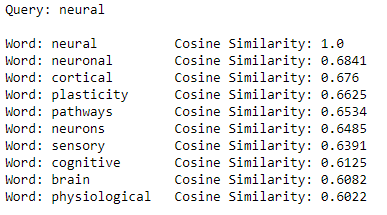
Embeddings are learned which means the representations apply specifically to one task. When using pre-trained embeddings, we hope the task the embeddings were learned on is close enough to our task so the embeddings are meaningful. If these embeddings were trained on tweets, we might not expect them to work well, but since they were trained on Wikipedia data, they should be generally applicable to a range of language processing tasks.

If you have a lot of data and the computer time, it’s usually better to learn your own embeddings for a specific task. In the notebook I take both approaches and the learned embeddings perform slightly better.

Training the Model

With the training and validation data prepared, the network built, and the embeddings loaded, we are almost ready for our model to learn how to write patent abstracts. However, good steps to take when training neural networks are to use ModelCheckpoint and EarlyStopping in the form of Keras callbacks:

• Model Checkpoint: saves the best model (as measured by validation loss) on disk for using best model
• Early Stopping: halts training when validation loss is no longer decreasing

Using Early Stopping means we won’t overfit to the training data and waste time training for extra epochs that don’t improve performance. The Model Checkpoint means we can access the best model and, if our training is disrupted 1000 epochs in, we won’t have lost all the progress!

from keras.callbacks import EarlyStopping, ModelCheckpoint

# Create callbacks
callbacks = [EarlyStopping(monitor='val_loss', patience=5),
             ModelCheckpoint('../models/model.h5'), save_best_only=True, 
                             save_weights_only=False)]

The model can then be trained with the following code:

history = model.fit(X_train,  y_train, 
                    batch_size=2048, epochs=150,
                    callbacks=callbacks,
                    validation_data=(X_valid, y_valid))

On an Amazon p2.xlarge instance ($0.90 / hour reserved), this took just over 1 hour to finish. Once the training is done, we can load back in the best saved model and evaluate a final time on the validation data.

from keras import load_model
# Load in model and evaluate on validation data
model = load_model('../models/model.h5')
model.evaluate(X_valid, y_valid)

Overall, the model using pre-trained word embeddings achieved a validation accuracy of 23.9%. This is pretty good considering as a human I find it extremely difficult to predict the next word in these abstracts! A naive guess of the most common word (“the”) yields an accuracy around 8%. The metrics for all the models in the notebook are shown below:

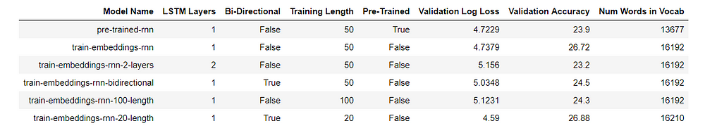
The best model used pre-trained embeddings and the same architecture as shown above. I’d encourage anyone to try training with a different model!

Patent Abstract Generation

Of course, while high metrics are nice, what matters is if the network can produce reasonable patent abstracts. Using the best model we can explore the model generation ability. If you want to run this on your own hardware, you can find the notebook here and the pre-trained models are on GitHub.

To produce output, we seed the network with a random sequence chosen from the patent abstracts, have it make a prediction of the next word, add the prediction to the sequence, and continue making predictions for however many words we want. Some results are shown below:

One important parameter for the output is the diversity of the predictions. Instead of using the predicted word with the highest probability, we inject diversity into the predictions and then choose the next word with a probability proportional to the more diverse predictions. Too high a diversity and the generated output starts to seem random, but too low and the network can get into recursive loops of output.

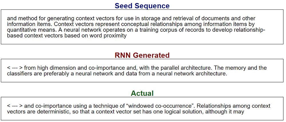
The output isn’t too bad! Some of the time it’s tough to determine which is computer generated and which is from a machine. Part of this is due to the nature of patent abstracts which, most of the time, don’t sound like they were written by a human.

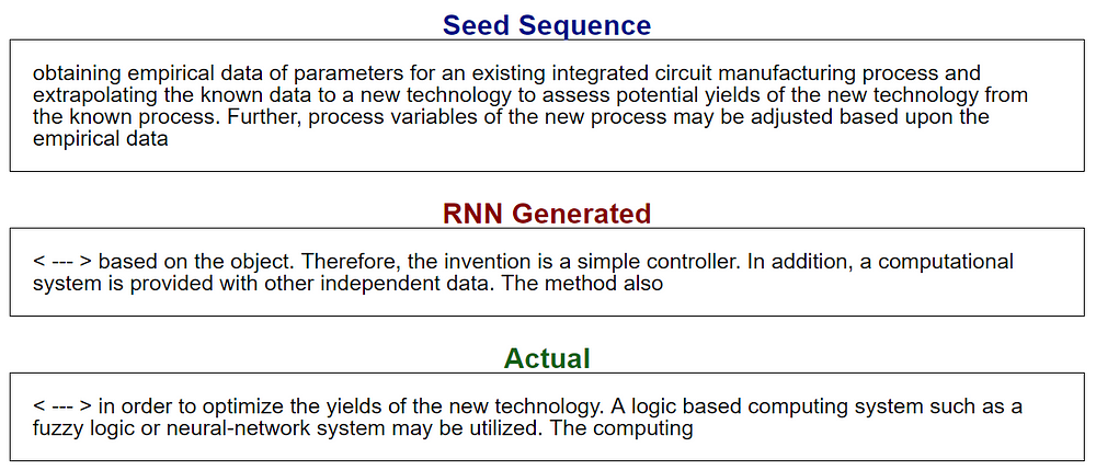
Another use of the network is to seed it with our own starting sequence. We can use any text we want and see where the network takes it:

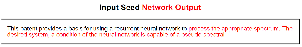
Again, the results are not entirely believable but they do resemble English.

Human or Machine?

As a final test of the recurrent neural network, I created a game to guess whether the model or a human generated the output. Here’s the first example where two of the options are from a computer and one is from a human:

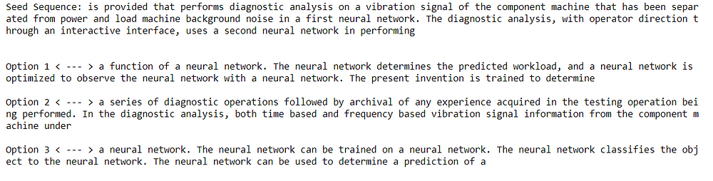
What’s your guess? The answer is that the second is the actual abstract written by a person (well, it’s what was actually in the abstract. I’m not sure these abstracts are written by people). Here’s another one:

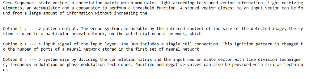
This time the third had a flesh and blood writer.

There are additional steps we can use to interpret the model such as finding which neurons light up with different input sequences. We can also look at the learned embeddings (or visualize them with the Projector tool). We’ll leave those topics for another time, and conclude that we know now how to implement a recurrent neural network to effectively mimic human text.

Conclusions

It’s important to recognize that the recurrent neural network has no concept of language understanding. It is effectively a very sophisticated pattern recognition machine. Nonetheless, unlike methods such as Markov chains or frequency analysis, the rnn makes predictions based on the ordering of elements in the sequence. Getting a little philosophical here, you could argue that humans are simply extreme pattern recognition machines and therefore the recurrent neural network is only acting like a human machine.

The uses of recurrent neural networks go far beyond text generation to machine translation, image captioning, and authorship identification. Although this application we covered here will not displace any humans, it’s conceivable that with more training data and a larger model, a neural network would be able to synthesize new, reasonable patent abstracts.

It can be easy to get stuck in the details or the theory behind a complex technique, but a more effective method for learning data science tools is to dive in and build applications. You can always go back later and catch up on the theory once you know what a technique is capable of and how it works in practice. Most of us won’t be designing neural networks, but it’s worth learning how to use them effectively. This means putting away the books, breaking out the keyboard, and coding up your very own network.

As always, I welcome feedback and constructive criticism. I can be reached on Twitter @koehrsen_will or through my website at willk.online.

30s ad

☞ The Python Video Workbook: Solve 100 Exercises

☞ Python 3: A Beginners Quick Start Guide to Python

☞ Learn the essentials of Python and ArcGIS’s arcpy

☞ The Developers Guide to Python 3 Programming

Suggest:

☞ Python Machine Learning Tutorial (Data Science)

☞ Python Tutorial for Data Science

☞ Machine Learning Zero to Hero - Learn Machine Learning from scratch

☞ Learn Python in 12 Hours | Python Tutorial For Beginners

☞ Complete Python Tutorial for Beginners (2019)

☞ What is Python and Why You Must Learn It in [2019]