How to get started with Machine Learning in about 10 minutes

With the rise of Machine Learning inside industries, the need for a tool that can help you iterate through the process quickly has become vital. Python, a rising star in Machine Learning technology, is often the first choice to bring you success. So, a guide to Machine Learning with Python is really necessary.

Introduction to Machine Learning with Python

So, why Python? In my experience, Python is one of the easiest programming languages to learn. There is a need to iterate the process quickly, and the data scientist does not need to have a deep knowledge of the language, as they can get the hang of it real quick.

How easy?

for anything in the_list:
    print(anything)

That easy. The syntax is closely related to English (or human language, not a machine). And there are no silly curly brackets that confuse humans. I have a colleague who is in Quality Assurance, not a Software Engineer, and she can write Python code within a day on production level. (For real!)

So the builders of the libraries we’ll discuss below chose Python for their choice of language. And as a Data Analyst and Scientist, we can just use their masterpieces to help us complete the tasks. These are the incredible libraries, that are must-haves for Machine Learning with Python.

Numpy

The famous numerical analysis library. It will help you do many things, from computing the median of data distribution, to processing multidimensional arrays.

2. Pandas

For processing CSV files. Of course, you will need to process some tables, and see statistics, and this is the right tool you want to use.

3. Matplotlib

After you have the data stored in Pandas data frames, you might need some visualizations to understand more about the data. Images are still better than thousands of words.

4. Seaborn

This is also another visualization tool, but more focused on statistical visualization. Things like histograms, or pie charts, or curves, or maybe correlation tables.

5. Scikit-Learn

This is the final boss of Machine Learning with Python. THE SO-CALLED Machine Learning with Python is this guy. Scikit-Learn. All of the things you need from algorithms to improvements are here.

6. Tensorflow and Pytorch

I don’t talk too much about these two. But if you are interested in Deep Learning, take a look at them, it will be worth your time. (I will give another tutorial about Deep Learning next time, stay tuned!)

Python Machine Learning Projects

Of course, reading and studying alone will not bring you where you need to go. You need actual practice. As I said on my blog, learning the tools is pointless if you do not jump into the data. And so, I introduce you to a place where you can find Python Machine Learning Projects easily.

Kaggle is a platform where you can dive directly into the data. You’ll solve projects and get really good at Machine Learning. Something that might make you more interested in it: the Machine Learning competitions it holds may give a prize as big as $100,000. And you might want to try your luck. Haha.

But, the most important thing is not the money — it is really a place where you can find Machine Learning with Python Projects. There are lots of projects you can try. But if you are a newbie, and I assume you are, you will want to join this competition.

Here’s an example project that we’ll use in the below tutorial:

Titanic: Machine Learning from Disaster

Yes, the infamous Titanic. A tragic disaster in 1912, that took the lives of 1502 people from 2224 passengers and crew. This Kaggle competition (or I can say tutorial) gives you the real data about the disaster. And your task is to explain the data so that you can predict whether a personal survived or not during the incident.

Machine Learning with Python Tutorial

Before going deep into the data of the Titanic, let’s install some tools you need.

Of course, Python. You need to install it first from the Python offfical website. You need to install version 3.6+ to keep up to date with the libraries.

After that, you need to install all the libraries via Python pip. Pip should be installed automatically with the distribution of Python you just downloaded.

Then install the things you need via pip. Open your terminal, command line, or Powershell, and write the following:

pip install numpypip install pandaspip install matplotlibpip install seabornpip install scikit-learnpip install jupyter

Well, everything looks good. But wait, what is jupyter? Jupyter stands for Julia, Python, and R, hence Jupytr. But it’s an odd combo of words, so they changed it into just Jupyter. It is a famous notebook where you can write Python code interactively.

Just type jupyter notebook in your terminal and you will open a browser page like this:

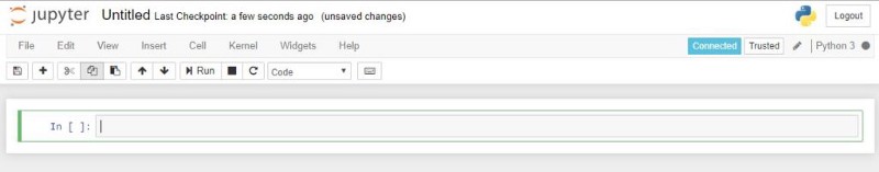
Write the code inside the green rectangle and you can write and evaluate Python code interactively.

Now you have installed all the tools. Let’s get going!

Data Exploration

The first step is to explore the data. You need to download the data from the Titanic page in Kaggle. Then put the extracted data inside a folder where you start your Jupyter notebook.

Then import the necessary libraries:

import numpy as np 
import pandas as pd
import matplotlib.pyplot as plt
import seaborn as sns
import warnings
warnings.filterwarnings('ignore')
%matplotlib inline

Then load the data:

train_df=pd.read_csv("train.csv")
train_df.head()

You will see something like this:

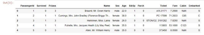
That is our data. It has the following columns:

PassengerId, the identifier of the passenger
Survived, whether he/she survived or not
Pclass, the class of the service, maybe 1 is economy, 2 is business, and 3 is first class
Name, the name of the passenger
Sex
Age
Sibsp, or siblings and spouses, number of siblings and spouses on board
Parch, or parents and children, number of them on board
Ticket, ticket detail
Cabin, their cabin. NaN means unknown
Embarked, the origin of embarkation, S for Southampton, Q for Queenstown, C for Cherbourg

While exploring data, we often find missing data. Let’s see them:

def missingdata(data):
    total = data.isnull().sum().sort_values(ascending = False)
    percent = (data.isnull().sum()/data.isnull().count()*100).sort_values(ascending = False)
    ms=pd.concat([total, percent], axis=1, keys=['Total', 'Percent'])
    ms= ms[ms["Percent"] > 0]
    f,ax =plt.subplots(figsize=(8,6))
    plt.xticks(rotation='90')
    fig=sns.barplot(ms.index, ms["Percent"],color="green",alpha=0.8)
    plt.xlabel('Features', fontsize=15)
    plt.ylabel('Percent of missing values', fontsize=15)
    plt.title('Percent missing data by feature', fontsize=15)
    return ms

missingdata(train_df)

We will see a result like this:

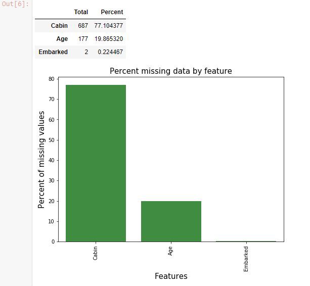
The cabin, age, and embarked data has some missing values. And cabin information is largely missing. We need to do something about them. This is what we call Data Cleaning.

Data Cleaning

This is what we use 90% of the time. We will do Data Cleaning a lot for every single Machine Learning project. When the data is clean, we can easily jump ahead to the next step without worrying about anything.

The most common technique in Data Cleaning is filling missing data. You can fill the data missing with Mode, Mean, or Median. There is no absolute rule on these choices — you can try to choose one after another and see the performance. But, for a rule of thumb, you can only use mode for categorized data, and you can use median or mean for continuous data.

So let’s fill the embarkation data with Mode and the Age data with median.

train_df['Embarked'].fillna(train_df['Embarked'].mode()[0], inplace = True)
train_df['Age'].fillna(train_df['Age'].median(), inplace = True)

The next important technique is to just remove the data, especially for largely missing data. Let’s do it for the cabin data.

drop_column = ['Cabin']
train_df.drop(drop_column, axis=1, inplace = True)

Now we can check the data we have cleaned.

print('check the nan value in train data')
print(train_df.isnull().sum())

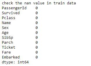
Perfect! No missing data found. Means the data has been cleaned.

Feature Engineering

Now we have cleaned the data. The next thing we can do is Feature Engineering.

Feature Engineering is basically a technique for finding Feature or Data from the currently available data. There are several ways to do this technique. More often, it is about common sense.

Let’s take a look at the Embarked data: it is filled with Q, S, or C. The Python library will not be able to process this, since it is only able to process numbers. So you need to do something called One Hot Vectorization, changing the column into three columns. Let’s say Embarked_Q, Embarked_S, and Embarked_C which are filled with 0 or 1 whether the person embarked from that harbor or not.

The other example is SibSp and Parch. Maybe there is nothing interesting in both of those columns, but you might want to know how big the family was of the passenger who boarded in the ship. You might assume that if the family was bigger, then the chance of survival would increase, since they could help each other. On other hand, solo people would’ve had it hard.

So you want to create another column called family size, which consists of sibsp + parch + 1 (the passenger themself).

The last example is called bin columns. It is a technique which creates ranges of values to group several things together, since you assume it is hard to differentiate things with similar value. For example, Age. For a person aged 5 and 6, is there any significant difference? or for person aged 45 and 46, is there any big difference?

That’s why we create bin columns. Maybe for age, we will create 4 bins. Children (0–14 years), Teenager (14–20), Adult (20–40), and Elders (40+)

Let’s code them:

all_data = train_df

for dataset in all_data :
    dataset['FamilySize'] = dataset['SibSp'] + dataset['Parch'] + 1

import re
# Define function to extract titles from passenger names
def get_title(name):
    title_search = re.search(' ([A-Za-z]+)\.', name)
    # If the title exists, extract and return it.
    if title_search:
        return title_search.group(1)
    return ""
# Create a new feature Title, containing the titles of passenger names
for dataset in all_data:
    dataset['Title'] = dataset['Name'].apply(get_title)
# Group all non-common titles into one single grouping "Rare"
for dataset in all_data:
    dataset['Title'] = dataset['Title'].replace(['Lady', 'Countess','Capt', 'Col','Don', 
                                                 'Dr', 'Major', 'Rev', 'Sir', 'Jonkheer', 'Dona'], 'Rare')

    dataset['Title'] = dataset['Title'].replace('Mlle', 'Miss')
    dataset['Title'] = dataset['Title'].replace('Ms', 'Miss')
    dataset['Title'] = dataset['Title'].replace('Mme', 'Mrs')

for dataset in all_data:
    dataset['Age_bin'] = pd.cut(dataset['Age'], bins=[0,14,20,40,120], labels=['Children','Teenage','Adult','Elder'])

for dataset in all_data:
    dataset['Fare_bin'] = pd.cut(dataset['Fare'], bins=[0,7.91,14.45,31,120], labels ['Low_fare','median_fare', 'Average_fare','high_fare'])
                                                                                
traindf=train_df
for dataset in traindf:
    drop_column = ['Age','Fare','Name','Ticket']
    dataset.drop(drop_column, axis=1, inplace = True)

drop_column = ['PassengerId']
traindf.drop(drop_column, axis=1, inplace = True)
traindf = pd.get_dummies(traindf, columns = ["Sex","Title","Age_bin","Embarked","Fare_bin"],
                             prefix=["Sex","Title","Age_type","Em_type","Fare_type"])

Now, you have finished all the features. Let’s take a look into the correlation for each feature:

sns.heatmap(traindf.corr(),annot=True,cmap='RdYlGn',linewidths=0.2) #data.corr()-->correlation matrix
fig=plt.gcf()
fig.set_size_inches(20,12)
plt.show()

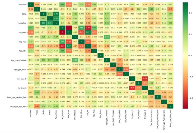
Correlations with value of 1 means highly correlated positively, -1 means highly correlated negatively. For example, sex male and sex female will correlate negatively, since passengers had to identify as one or the other sex. Other than that, you can see that nothing related to anything highly except for the ones created via feature engineering. This means we are good to go.

What will happen if something highly correlates with something else? We can eliminate one of them since adding nother information via a new column will not give the system new information since both of them are exactly the same.

Machine Learning with Python

Now we have arrived at the apex of the tutorial: Machine Learning modeling.

from sklearn.model_selection import train_test_split #for split the data
from sklearn.metrics import accuracy_score  #for accuracy_score
from sklearn.model_selection import KFold #for K-fold cross validation
from sklearn.model_selection import cross_val_score #score evaluation
from sklearn.model_selection import cross_val_predict #prediction
from sklearn.metrics import confusion_matrix #for confusion matrix
all_features = traindf.drop("Survived",axis=1)
Targeted_feature = traindf["Survived"]
X_train,X_test,y_train,y_test = train_test_split(all_features,Targeted_feature,test_size=0.3,random_state=42)
X_train.shape,X_test.shape,y_train.shape,y_test.shape

You can choose many algorithms included inside the scikit-learn library.

Logistic Regression
Random Forest
SVM
K Nearest Neighbor
Naive Bayes
Decision Trees
AdaBoost
LDA
Gradient Boosting

You might be overwhelmed trying to figure out what is what. Don’t worry, just treat is as a black box: choose one with the best performance. (I will create a whole article on these algorithms later.)

Let’s try it with my favorite one: the Random Forest Algorithm

from sklearn.ensemble import RandomForestClassifier
model = RandomForestClassifier(criterion='gini', n_estimators=700,
                             min_samples_split=10,min_samples_leaf=1,
                             max_features='auto',oob_score=True,
                             random_state=1,n_jobs=-1)
model.fit(X_train,y_train)
prediction_rm=model.predict(X_test)
print('--------------The Accuracy of the model----------------------------')
print('The accuracy of the Random Forest Classifier is', round(accuracy_score(prediction_rm,y_test)*100,2))
kfold = KFold(n_splits=10, random_state=22) # k=10, split the data into 10 equal parts
result_rm=cross_val_score(model,all_features,Targeted_feature,cv=10,scoring='accuracy')
print('The cross validated score for Random Forest Classifier is:',round(result_rm.mean()*100,2))
y_pred = cross_val_predict(model,all_features,Targeted_feature,cv=10)
sns.heatmap(confusion_matrix(Targeted_feature,y_pred),annot=True,fmt='3.0f',cmap="summer")
plt.title('Confusion_matrix', y=1.05, size=15)

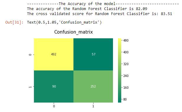
Wow! It gives us 83% accuracy. That’s good enough for our first time.

The cross validated score means a K Fold Validation method. If K = 10, it means you split the data in 10 variations and compute the mean of all scores as the final score.

Fine Tuning

Now you are done with the steps in Machine Learning with Python. But, there is one more step which can bring you better results: fine tuning. Fine tuning means finding the best parameter for Machine Learning Algorithms. If you see the code for random forest above:

model = RandomForestClassifier(criterion='gini', n_estimators=700,
                             min_samples_split=10,min_samples_leaf=1,
                             max_features='auto',oob_score=True,
                             random_state=1,n_jobs=-1)

There are many parameters you need to set. These are the defaults, by the way. And you can change the parameters however you want. But of course, it will takes a lot of time.

Don’t worry — there is a tool called Grid Search, which finds the optimal parameters automatically. Sounds great, right?

# Random Forest Classifier Parameters tunning 
model = RandomForestClassifier()
n_estim=range(100,1000,100)

## Search grid for optimal parameters
param_grid = {"n_estimators" :n_estim}


model_rf = GridSearchCV(model,param_grid = param_grid, cv=5, scoring="accuracy", n_jobs= 4, verbose = 1)

model_rf.fit(train_X,train_Y)

# Best score
print(model_rf.best_score_)

#best estimator
model_rf.best_estimator_

Well, you can try it out for yourself. And have fun with Machine Learning.

Conclusion

How was it? It doesn’t seem very difficult does it? Machine Learning with Python is easy. Everything has been laid out for you. You can just do the magic. And bring happiness to people.

This piece was originally released on my blog at thedatamage.com

✅ 30s ad

☞ Machine Learning Guide: Learn Machine Learning Algorithms

☞ Introduction to Machine Learning & Deep Learning in Python

☞ Hands-On Machine Learning: Learn TensorFlow, Python, & Java!

☞ Learn Azure Machine Learning from scratch

☞ Master Machine Learning , Deep Learning with Python

Suggest:

☞ Machine Learning Zero to Hero - Learn Machine Learning from scratch

☞ Learn Python in 12 Hours | Python Tutorial For Beginners

☞ Complete Python Tutorial for Beginners (2019)

☞ What is Python and Why You Must Learn It in [2019]

☞ Python Machine Learning Tutorial (Data Science)

☞ Python Programming Tutorial | Full Python Course for Beginners 2019