The ABC of Machine Learning

The Buzz around Machine Learning has developed keen interest among the techies to get their hands on ML. However, before diving into the ocean of ML here are few basic concepts that you should be familiar with. Keep this handy as you will come across these terms frequently while learning ML.
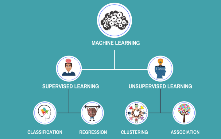
Supervised, Unsupervised and Semi-Supervised Learning:
Supervised Learning:
Supervised learning as the name indicates the presence of a supervisor as a teacher. Basically supervised learning is a learning in which we teach or train the machine using data which is well labeled that means the data is already tagged with the correct answer. After that, the machine is provided with the new set of examples(data) without the target label (desired output) and machine predicts the output of the new data by applying its learning from historical trained data.
Supervised learning is where you have input variables (x) and an output variable (Y) and you use an algorithm to learn the mapping function from the input to the output.
Y = f(X)
The goal is to approximate the mapping function so well that when you have new input data (x) that you can predict the output variables (Y) for that data.
Supervised learning problems can be further grouped into regression and classification problems.
· Classification: A classification problem is when the output variable is a category, such as “red” or “blue” or “disease” and “no disease”.
· Regression: A regression problem is when the output variable is a real value, such as “Salary” or “Price”.
Unsupervised Learning:
Unsupervised learning is where you only have input data (X) and no corresponding output variables.
The goal for unsupervised learning is to model the underlying structure or distribution in the data in order to learn more about the data.
These are called unsupervised learning because unlike supervised learning above there are no correct answers and there is no teacher. Algorithms are left to their own devices to discover and present the interesting structure in the data.
Unsupervised learning problems can be further grouped into clustering and association problems.
· Clustering: A clustering problem is where you want to discover the inherent groupings in the data, such as grouping customers by purchasing behavior.
· Association: An association rule learning problem is where you want to discover rules that describe large portions of your data, such as people that buy X also tend to buy Y.
Some popular examples of unsupervised learning algorithms are:
· k-means for clustering problems.
· Apriori algorithm for association rule learning problems.
Semi-Supervised Learning:
Problems where you have a large amount of input data (X) and only some of the data is labeled (Y) are called semi-supervised learning problems.
These problems sit in between both supervised and unsupervised learning.
A good example is a photo archive where only some of the images are labeled, (e.g. dog, cat, person) and the majority are unlabeled.
Many real-world machine learning problems fall into this area. This is because it can be expensive or time-consuming to label data as it may require access to domain experts. Whereas unlabeled data is cheap and easy to collect and store.
You can use unsupervised learning techniques to discover and learn the structure in the input variables.
You can also use supervised learning techniques to make best guess predictions for the unlabeled data, feed that data back into the supervised learning algorithm as training data and use the model to make predictions on new unseen data.
Categorical and Continuous features in Machine Learning:
Features are the term used for the columns in the analytics base table (ABT). All features can be classified as either categorical or continuous. Categorical features have one of few values, where the choices are categories (such as less than 50 or greater than 50), Fraud or Not Fraud, Credit Card Default or Not Default etc whereas Continuous features have many possible options for values like Salary of Person, Age of a Person, Price of a commodity, Loan Amount to be given etc.
If categorical features are other than number or string then it needs to be encoded into its numeric representation either by manual replacement, Label Encoder or One Hot Encoderas ML models can only process numbers and not string values
Scikit-learn:
Scikit-learn is probably the most useful library for machine learning in Python. Scikit-learn provides a range of supervised and unsupervised learning algorithms via a consistent interface in Python. Scikit-learn comes loaded with a lot of features. Consider Scikit-learn as a toolbox for Machine Learning. Here are a few of them to help you understand the spread:
· Supervised learning algorithms: Think of any supervised learning algorithm you might have heard about and there is a very high chance that it is part of scikit-learn. Starting from Generalized linear models (e.g Linear Regression), Support Vector Machines (SVM), Decision Trees to Bayesian methods — all of them are part of scikit-learn toolbox. The spread of algorithms is one of the big reasons for the high usage of scikit-learn. I started using scikit to solve supervised learning problems and would recommend that to people new to scikit / machine learning as well.
· Cross-validation: There are various methods to check the accuracy of supervised models on unseen data
· Unsupervised learning algorithms: Again there is a large spread of algorithms in the offering — starting from clustering, factor analysis, principal component analysis to unsupervised neural networks.
· Various toy datasets: This came in handy while learning scikit-learn (e.g. IRIS dataset, Boston House prices dataset). Having them handy while learning a new library helps a lot.
· Feature extraction: Useful for extracting features from images, text (e.g. Bag of words)
Training and Testing Datasets:
Training Dataset:
Training Dataset is the part of Original Dataset that we use to train our ML model. The model learns on this data by running the algorithm and maps a function F(x) where “x” in the independent variable (inputs) for “y” where “y” is the dependent variable(output). While Training our model on a dataset we provide both input and output variables to our model so that our model is able to learn to predict the output based on the input data.
Testing Data:
Testing data is basically the validation set which has been reserved from the original dataset, it is used to check the accuracy of our model by comparing the predicted outcome of the model to the actual outcome of the test dataset. We do not provide output variable to our model while testing although we know the outcome as Test data is extracted from the original dataset itself. When the model gives us its predictions based on the learning from the training data we compare the predicted outcome with the original outcome to get the measure of accuracy or performance of our model on unseen data.
Consider an Example where our Original Dataset has 1000 rows and our dependent variable is Fraud and Not Fraud, we will train our model on 70% of data i.e 700 rows and then test our model accuracy on 30% of data i.e 300 rows. As discussed above while testing our model we will not provide the outcome to our model for the test data although we know the outcome and let our model will give us the outcome for those 300 rows and later we will compare the outcome of our model to the original outcome of our test data to get the accuracy of our model predictions.
For splitting our data to training and testing set we use train_test_split method of scikit-learn library
Confusion Matrix:
Confusion Matrix is the measure of correctness of the predictions made by the Classification model.
As the name suggests Confusion Matrix is a matrix representation of correct and incorrect predictions made by the model.
Consider a scenario where we predict whether the person is suffering from a “Disease” (event) or “No Disease” (no event).
Confusion matrix now will be made based on 4 terms
· “true positive” for correctly predicted event values.
· “false positive” for incorrectly predicted event values.
· “true negative” for correctly predicted no-event values.
· “false negative” for incorrectly predicted no-event values.
Let’s suppose we have 100 testing data out of which 50 has Disease (D) and 50 No Disease (ND) and our model predicted the outcome as 45 Disease (D) and 55 No Disease, in this case, our confusion matrix will be

true positive: 45.
false positive: 5 (Total event values — Predicted event values i.e 50–45)
true negative: 50 (Total values — Total No event values i.e 100–50)
false negative: 0
Green diagonal represents correct predictions and red diagonal represents incorrect predictions hence the total number of correct predictions is 45+50 = 95
And incorrect predictions is 5+0 = 5
Accuracy Score:
Accuracy score also provides the measure of accuracy or correctness of the predictions made by classification model but it is a between a range of 0 to 1 which is then multiplied by 100 to get a score between 0 to 100, closer the value to 1 more accurate is the model.
Accuracy score is Calculated as :
Accuracy score = Total Correct Predictions/Total Predictions made * 100
Considering the previous scenario accuracy score will be =
95/100 * 100 = 0.95*100 = 95%
library used for calculating accuracy score is sklearn.metrics.accuracy_score

Mean Absolute Error and Root Mean Squared Error:
While Classification models can be very well evaluated using Accuracy Score and Confusion Matrix, regression models are evaluated using Mean Absolute Error and Root Mean Squared Error as the aim of our regression model is to predict values as close as to the actual values.
Closer the MAE and RMSE to 0 more accurate is the model.
Mean Absolute Error:
It is calculated as the average of the absolute error values, where “absolute” means “made positive” so that they can be added together.
MAE = sum( abs(predicted- actual ) / total predictions
Consider an Example;
Actual Values = [2,4,6,8] , Predicted Values = [4,6,8,10]
MAE = abs(4–2 + 6–4 + 8–6 + 10–8)/4 = 2
library used for calculating mean absolute error is sklearn.metrics.mean_absolute_error
Root Mean Squared Error:
Another popular way to calculate the error in a set of regression predictions is to use the Root Mean Squared Error.
Shortened as RMSE, the metric is sometimes called Mean Squared Error or MSE, dropping the Root part from the calculation and the name.
RMSE is calculated as the square root of the mean of the squared differences between actual outcomes and predictions.
Squaring each error forces the values to be positive, and the square root of the mean squared error returns the error metric back to the original units for comparison.
RMSE = sqrt( sum( (predicted- actual)²) / total predictions)
Actual Values = [2,4,6,8] , Predicted Values = [4,6,8,10]
RMSE = sqrt((8)²/4) = sqrt(64/4) = sqrt(16) = 4
Once you are familiar with the above terms and have basic knowledge of python you are ready to get your hands dirty with trying out some simple ML models.
If this blog has helped you give some **CLAPS**and SHARE it with your friends.
— Thank You
30s ad
☞ Data Science and Machine Learning for Managers and MBAs
☞ Cluster Analysis: Unsupervised Machine Learning with Python
☞ Machine Learning In The Cloud With Azure Machine Learning
☞ R Machine Learning solutions
☞ A-Z Machine Learning using Azure Machine Learning (AzureML)
Suggest:
☞ Python Machine Learning Tutorial (Data Science)
☞ Python Tutorial for Data Science
☞ Machine Learning Zero to Hero - Learn Machine Learning from scratch
☞ Learn Python in 12 Hours | Python Tutorial For Beginners