Explored Deep Learning Through 6 Code Snippets

The History of Deep Learning — Explored Through 6 Code Snippets
In this article, we’ll explore six snippets of code that made deep learning what it is today. We’ll cover the inventors and the background to their breakthroughs. Each story includes simple code samples on FloydHub and GitHub to play around with.
If this is your first encounter with deep learning, I’d suggest reading my Deep Learning 101 for Developers.
To run the code examples on FloydHub, install the floydcommand line tool. Then clone the code examples I’ve provided to your local machine.
Note: If you are new to FloydHub, you might want to first read the getting started with FloydHub section in my earlier post.
Initiate the CLI in the example project folder on your local machine. Now you can spin up the project on FloydHub with the following command:
floyd run --data emilwallner/datasets/mnist/1:mnist --tensorboard --mode jupyter
The Method of Least Squares
Deep learning started with a snippet of math.
I’ve translated it into Python:
# y = mx + b
# m is slope, b is y-intercept
def compute_error_for_line_given_points(b, m, coordinates):
    totalError = 0
    for i in range(0, len(coordinates)):
        x = coordinates[i][0]
        y = coordinates[i][1]
        totalError += (y - (m * x + b)) ** 2
    return totalError / float(len(coordinates))
# example
compute_error_for_line_given_points(1, 2, [[3,6],[6,9],[12,18]])
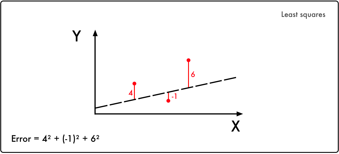
This was first published by Adrien-Marie Legendre in 1805. He was a Parisian mathematician who was also known for measuring the meter.
He had a particular obsession with predicting the future location of comets. He had the locations of a couple of past comets. He was relentless as he used them in his search for a method to calculate their trajectory.
It really was one of those spaghetti-on-the-wall moments. He tried several methods, then one version finally stuck with him.
Legendre’s process started by guessing the future location of a comet. Then he squared the errors he made, and finally remade his guess to reduce the sum of the squared errors. This was the seed for linear regression.
Play with the above code in the Jupyter notebook I’ve provided to get a feel for it. mis the coefficient and b in the constant for your prediction, and the coordinates are the locations of the comet. The goal is to find a combination of m and b where the error is as small as possible.
This is the core of deep learning:
- Take an input and a desired output
- Then search for the correlation between the two
Gradient Descent
Legendre’s method of manually trying to reduce the error rate was time-consuming. Peter Debye was a Nobel prize winner from The Netherlands. He formalized a solution for this process a century later in 1909.
Let’s imagine that Legendre had one parameter to worry about — we’ll call it X. The Y axis represents the error value for each value of X. Legendre was searching for where X results in the lowest error.
In this graphical representation, we can see that the value of X that minimizes the error Y is when X = 1.1.
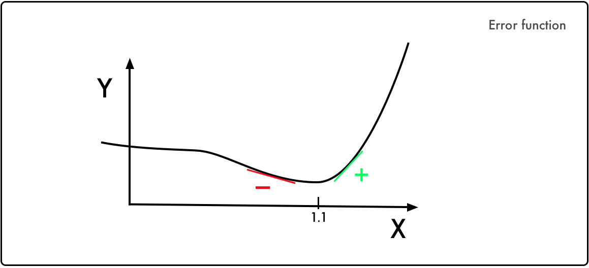
Peter Debye noticed that the slope to the left of the minimum is negative, while it’s positive on the other side. Thus, if you know the value of the slope at any given X value, you can guide Y towards its minimum.
This led to the method of gradient descent. The principle is used in almost every deep learning model.
To play with this, let’s assume that the error function is Error = x⁵ -2x³-2. To know the slope of any given X value we take its derivative, which is 5x⁴ - 6x²:

Watch Khan Academy’s video if you need to brush up your knowledge on derivatives.
Debye’s math translated into Python:
current_x = 0.5 # the algorithm starts at x=0.5
learning_rate = 0.01 # step size multiplier
num_iterations = 60 # the number of times to train the function
#the derivative of the error function (x**4 = the power of 4 or x^4)
def slope_at_given_x_value(x):
   return 5 * x**4 - 6 * x**2
# Move X to the right or left depending on the slope of the error function
for i in range(num_iterations):
   previous_x = current_x
   current_x += -learning_rate * slope_at_given_x_value(previous_x)
   print(previous_x)
print("The local minimum occurs at %f" % current_x)
The trick here is the learning_rate. By going in the opposite direction of the slope it approaches the minimum. Additionally, the closer it gets to the minimum, the smaller the slope gets. This reduces each step as the slope approaches zero.
num_iterations is your estimated time of iterations before you reach the minimum. Play with the parameters it to get an intuition for gradient descent.
Linear Regression
Combining the method of least square and gradient descent you get linear regression. In the 1950s and 1960s, a group of experimental economists implemented versions of these ideas on early computers. The logic was implemented on physical punch cards — truly handmade software programs. It took several days to prepare these punch cards and up to 24 hours to run one regression analysis through the computer.
Here’s a linear regression example translated into Python so that you don’t have to do it in punch cards:
#Price of wheat/kg and the average price of bread
wheat_and_bread = [[0.5,5],[0.6,5.5],[0.8,6],[1.1,6.8],[1.4,7]]
def step_gradient(b_current, m_current, points, learningRate):
    b_gradient = 0
    m_gradient = 0
    N = float(len(points))
    for i in range(0, len(points)):
        x = points[i][0]
        y = points[i][1]
        b_gradient += -(2/N) * (y - ((m_current * x) + b_current))
        m_gradient += -(2/N) * x * (y - ((m_current * x) + b_current))
    new_b = b_current - (learningRate * b_gradient)
    new_m = m_current - (learningRate * m_gradient)
    return [new_b, new_m]
def gradient_descent_runner(points, starting_b, starting_m, learning_rate, num_iterations):
    b = starting_b
    m = starting_m
    for i in range(num_iterations):
        b, m = step_gradient(b, m, points, learning_rate)
    return [b, m]
gradient_descent_runner(wheat_and_bread, 1, 1, 0.01, 100)
This should not introduce anything new. However, it can be a bit of a mind boggle to merge the error function with gradient descent. Run the code and play around with this linear regression simulator.
The Perceptron
Enter Frank Rosenblatt — the guy who dissected rat brains during the day and searched for signs of extraterrestrial life at night. In 1958, he hit the front page of New York Times: “New Navy Device Learns By Doing” with a machine that mimics a neuron.
If you showed Rosenblatt’s machine 50 sets of two images, one with a mark to the left and the other on the right, it could make the distinction without being pre-programmed. The public got carried away with the possibilities of a true learning machine.
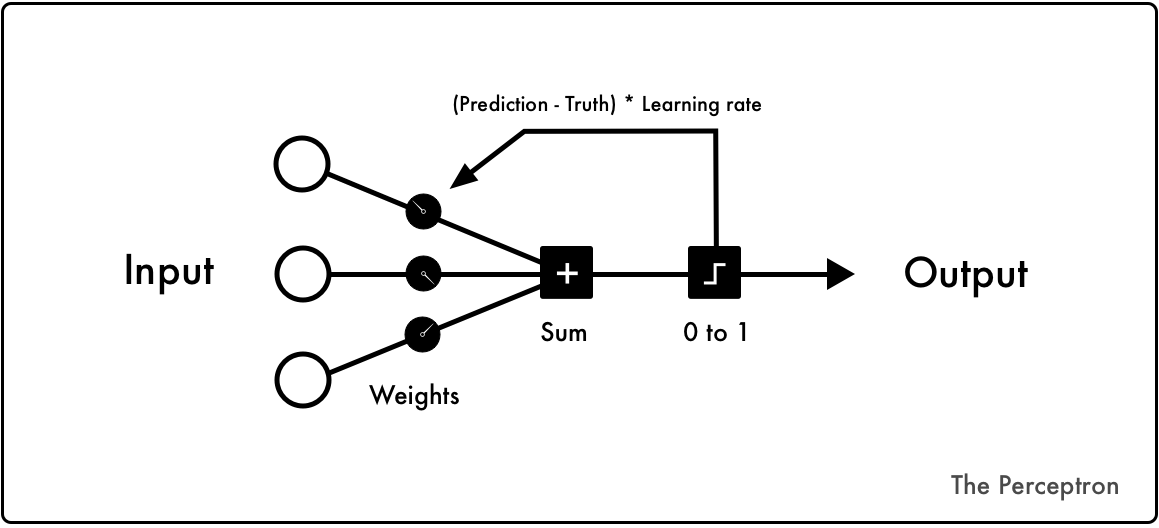
For every training cycle, you start with input data to the left. Initial random weights are added to all the input data. They are then summed up. If the sum is negative, it’s translated into 0, otherwise, it’s mapped into a 1.
If the prediction is correct, then nothing happens to the weights in that cycle. If it’s wrong, you multiply the error with a learning rate. This adjusts the weights accordingly.
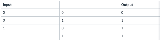
Let’s run the perceptron with the classic OR logic.
The perceptron machine translated into Python:
from random import choice
from numpy import array, dot, random
1_or_0 = lambda x: 0 if x < 0 else 1
training_data = [ (array([0,0,1]), 0),
                    (array([0,1,1]), 1),
                    (array([1,0,1]), 1),
                    (array([1,1,1]), 1), ]
weights = random.rand(3)
errors = []
learning_rate = 0.2
num_iterations = 100
for i in range(num_iterations):
    input, truth = choice(training_data)
    result = dot(weights, input)
    error = truth - 1_or_0(result)
    errors.append(error)
    weights += learning_rate * error * input

for x, _ in training_data:
    result = dot(x, w)
    print("{}: {} -> {}".format(input[:2], result, 1_or_0(result)))
In 1969, Marvin Minsky and Seymour Papert destroyed the idea. At the time, Minsky and Papert ran the AI lab at MIT. They wrote a book proving that the perceptron could only solve linear problems. They also debunked claims about the multi-layer perceptron. Sadly, Frank Rosenblatt died in a boat accident two years later.
In 1970 a Finnish master student, discovered the theory to solve non-linear problems with multi-layered perceptrons. Because of the mainstream criticism of the perceptron, the funding of AI dried up for more than a decade. This was known as the first AI winter.
The power of Minsky and Papert’s critique was the XOR problem. The logic is the same as the OR logic with one exception — when you have two true statements (1 & 1), you return False (0).
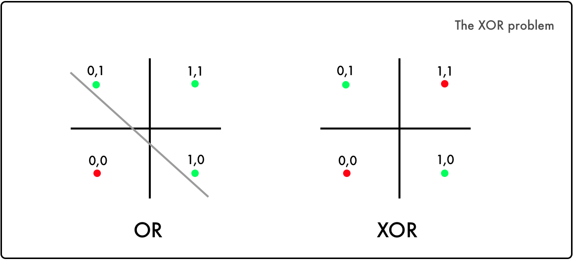
In the OR logic, it’s possible to divide the true combination from the false ones. But as you can see, you can’t divide the XOR logic with one linear function.
Artificial Neural Networks
By 1986, several experiments proved that neural networks could solve complex nonlinear problems. At the time, computers were 10,000 times faster compared to when the theory was developed. This is how Rumelhart introduced the legendary paper:
To understand the core of this paper, we’ll code the implementation by DeepMind’s Andrew Trask. This is not a random snippet of code. It’s been used in Andrew Karpathy’s deep learning course at Stanford and Siraj Raval’s Udacity course. It solves the XOR problem, thawing the first AI winter.
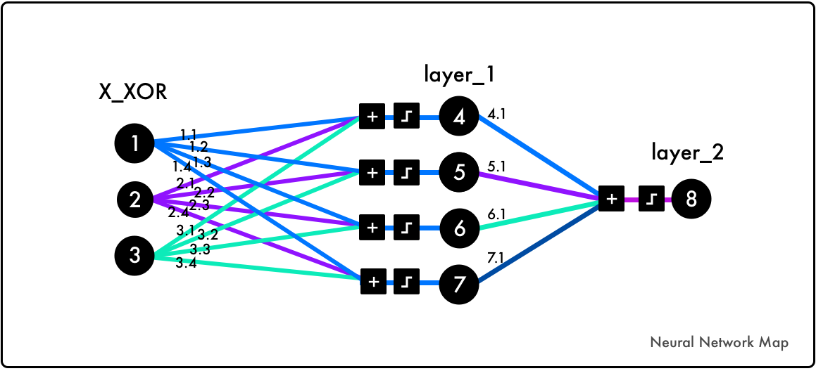
Before we dig into the code, play with this simulator for one to two hours to grasp the core logic. Then read Trask’s blog post.
Note that the added parameter [1] in the X_XOR data are bias neurons.
They have the same behavior as a constant in a linear function:
import numpy as np
X_XOR = np.array([[0,0,1], [0,1,1], [1,0,1],[1,1,1]])
y_truth = np.array([[0],[1],[1],[0]])
np.random.seed(1)
syn_0 = 2*np.random.random((3,4)) - 1
syn_1 = 2*np.random.random((4,1)) - 1
def sigmoid(x):
    output = 1/(1+np.exp(-x))
    return output
def sigmoid_output_to_derivative(output):
    return output*(1-output)
for j in range(60000):
    layer_1 = sigmoid(np.dot(X_XOR, syn_0))
    layer_2 = sigmoid(np.dot(layer_1, syn_1))
    error = layer_2 - y_truth
    layer_2_delta = error * sigmoid_output_to_derivative(layer_2)
    layer_1_error = layer_2_delta.dot(syn_1.T)
    layer_1_delta = layer_1_error * sigmoid_output_to_derivative(layer_1)
    syn_1 -= layer_1.T.dot(layer_2_delta)
    syn_0 -= X_XOR.T.dot(layer_1_delta)

print("Output After Training: \n", layer_2)
Backpropagation, matrix multiplication, and gradient descent combined can be hard to wrap your mind around. The visualizations of this process is often a simplification of what’s going on behind the hood. Focus on understanding the logic behind it, but don’t worry too much of having a mental picture of it.
Also, look at Andrew Karpathy’s lecture on backpropagation, play with these visualizations, and read Michael Nielsen’s chapter on it.
Deep Neural Networks
Deep neural networks are neural networks with more than one layer between the input and output layer. The notion was introduced by Rina Dechter in 1986. But it didn’t gain mainstream attention until 2012. This was soon after IBM Watson’s Jeopardy victory and Google’s cat recognizer.
The core structure of deep neural network have stayed the same. But they are now applied to several different problems. There have also been a lot of improvement in regularization.
In 1963, it was a set of math functions to simplify noisy earth data. They are now used in neural networks to improve their ability to generalize.
A large share of the innovation is due to computing power. This improved researcher’s innovation cycles — what took a supercomputer one year to calculate in the mid-eighties takes half a second with today’s GPU technology.
The reduced cost in computing and the development of deep learning libraries have now made it accessible to the general public. Let’s look at an example of a common deep learning stack, starting from the bottom layer:
- GPU > Nvidia Tesla K80. The hardware commonly used for graphics processing. Compared to CPUs, they are on average 50–200 times faster for deep learning.
- CUDA > low level programming language for the GPUs
- CuDNN > Nvidia’s library to optimize CUDA
- Tensorflow > Google’s deep learning framework on top of CuDNN
- TFlearn > A front-end framework for Tensorflow
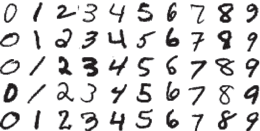
Let’s have a look at the MNIST image classification of digits, the “Hello World” of deep learning.
Implemented in TFlearn:
from __future__ import division, print_function, absolute_import
import tflearn
from tflearn.layers.core import dropout, fully_connected
from tensorflow.examples.tutorials.mnist import input_data
from tflearn.layers.conv import conv_2d, max_pool_2d
from tflearn.layers.normalization import local_response_normalization
from tflearn.layers.estimator import regression
# Data loading and preprocessing
mnist = input_data.read_data_sets("/data/", one_hot=True)
X, Y, testX, testY = mnist.train.images, mnist.train.labels, mnist.test.images, mnist.test.labels
X = X.reshape([-1, 28, 28, 1])
testX = testX.reshape([-1, 28, 28, 1])
# Building convolutional network
network = tflearn.input_data(shape=[None, 28, 28, 1], name='input')
network = conv_2d(network, 32, 3, activation='relu', regularizer="L2")
network = max_pool_2d(network, 2)
network = local_response_normalization(network)
network = conv_2d(network, 64, 3, activation='relu', regularizer="L2")
network = max_pool_2d(network, 2)
network = local_response_normalization(network)
network = fully_connected(network, 128, activation='tanh')
network = dropout(network, 0.8)
network = fully_connected(network, 256, activation='tanh')
network = dropout(network, 0.8)
network = fully_connected(network, 10, activation='softmax')
network = regression(network, optimizer='adam', learning_rate=0.01,
                        loss='categorical_crossentropy', name='target')
# Training
model = tflearn.DNN(network, tensorboard_verbose=0)
model.fit({'input': X}, {'target': Y}, n_epoch=20,
            validation_set=({'input': testX}, {'target': testY}),
            snapshot_step=100, show_metric=True, run_id='convnet_mnist')
There are plenty of great articles explaining the MNIST problem: here and here.
Let’s sum it up
As you see in the TFlearn example, the main logic of deep learning is still similar to Rosenblatt’s perceptron. Instead of using a binary Heaviside step function, today’s networks mostly use Relu (Rectifier linear unit) activations.
In the last layer of the convolutional neural network, loss equals categorical_crossentropy. This is an evolution of Legendre’s least square, a logistical regression for multiple categories. The optimizer adamoriginates from the work of Debye’ gradient descent.
Tikhonov’s regularization notion is widely implemented in the form of dropout layers and regularization functions, L1/L2.
**Recommended Courses: **
Machine Learning - Fun and Easy using Python and Keras
☞ https://goo.gl/vmmhvm
Machine Learning A-Z™: Hands-On Python & R In Data Science
☞ http://go.codetrick.net/HyqmWXWlz
Data Science: Master Machine Learning Without Coding
☞ https://goo.gl/3XF2yp
Complete Guide to TensorFlow for Deep Learning with Python
☞ http://go.codetrick.net/H1eF7ZQZgG
Suggest:
☞ Python Machine Learning Tutorial (Data Science)
☞ Python Tutorial for Data Science
☞ Machine Learning Zero to Hero - Learn Machine Learning from scratch
☞ Learn Python in 12 Hours | Python Tutorial For Beginners