Creating a Neural Network from Scratch in Python

Motivation: As part of my personal journey to gain a better understanding of Deep Learning, I’ve decided to build a Neural Network from scratch without a deep learning library like TensorFlow. I believe that understanding the inner workings of a Neural Network is important to any aspiring Data Scientist.
This article contains what I’ve learned, and hopefully it’ll be useful for you as well!
What’s a Neural Network?
Most introductory texts to Neural Networks brings up brain analogies when describing them. Without delving into brain analogies, I find it easier to simply describe Neural Networks as a mathematical function that maps a given input to a desired output.
Neural Networks consist of the following components
- An input layer, x
- An arbitrary amount of hidden layers
- An output layer, ŷ
- A set of weights and biases between each layer, W and b
- A choice of activation function for each hidden layer, σ. In this tutorial, we’ll use a Sigmoid activation function.
The diagram below shows the architecture of a 2-layer Neural Network (note that the input layer is typically excluded when counting the number of layers in a Neural Network)

Creating a Neural Network class in Python is easy.
neural_network_init.py
class NeuralNetwork:
    def __init__(self, x, y):
        self.input      = x
        self.weights1   = np.random.rand(self.input.shape[1],4)
        self.weights2   = np.random.rand(4,1)
        self.y          = y
        self.output     = np.zeros(y.shape)
Training the Neural Network
The output ŷ of a simple 2-layer Neural Network is:

You might notice that in the equation above, the weights W and the biases b are the only variables that affects the output ŷ.
Naturally, the right values for the weights and biases determines the strength of the predictions. The process of fine-tuning the weights and biases from the input data is known as training the Neural Network.
Each iteration of the training process consists of the following steps:
- Calculating the predicted output ŷ, known as feedforward
- Updating the weights and biases, known as backpropagation
The sequential graph below illustrates the process.
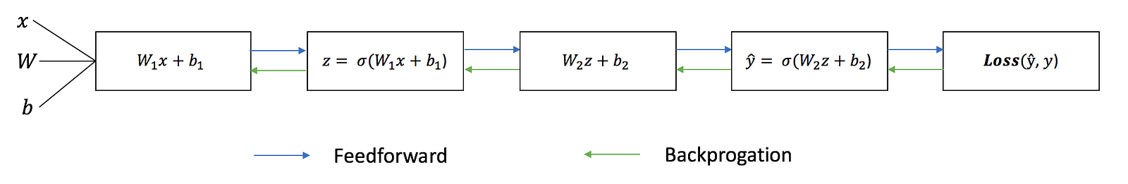
Feedforward
As we’ve seen in the sequential graph above, feedforward is just simple calculus and for a basic 2-layer neural network, the output of the Neural Network is:
Let’s add a feedforward function in our python code to do exactly that. Note that for simplicity, we have assumed the biases to be 0.
neural_network_feedforward.py
class NeuralNetwork:
    def __init__(self, x, y):
        self.input      = x
        self.weights1   = np.random.rand(self.input.shape[1],4)
        self.weights2   = np.random.rand(4,1)
        self.y          = y
        self.output     = np.zeros(self.y.shape)

    def feedforward(self):
        self.layer1 = sigmoid(np.dot(self.input, self.weights1))
        self.output = sigmoid(np.dot(self.layer1, self.weights2))
However, we still need a way to evaluate the “goodness” of our predictions (i.e. how far off are our predictions)? The Loss Function allows us to do exactly that.
Loss Function
There are many available loss functions, and the nature of our problem should dictate our choice of loss function. In this tutorial, we’ll use a simple sum-of-sqaures error as our loss function.
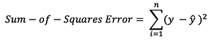
That is, the sum-of-squares error is simply the sum of the difference between each predicted value and the actual value. The difference is squared so that we measure the absolute value of the difference.
Our goal in training is to find the best set of weights and biases that minimizes the loss function.
Backpropagation
Now that we’ve measured the error of our prediction (loss), we need to find a way to propagate the error back, and to update our weights and biases.
In order to know the appropriate amount to adjust the weights and biases by, we need to know the derivative of the loss function with respect to the weights and biases.
Recall from calculus that the derivative of a function is simply the slope of the function.
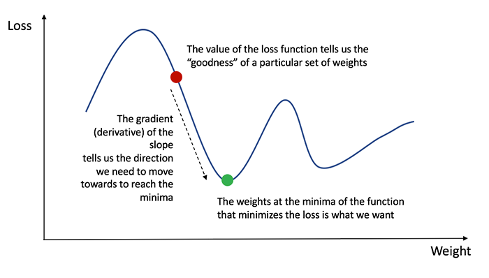
If we have the derivative, we can simply update the weights and biases by increasing/reducing with it(refer to the diagram above). This is known as gradient descent.
However, we can’t directly calculate the derivative of the loss function with respect to the weights and biases because the equation of the loss function does not contain the weights and biases. Therefore, we need the chain rule to help us calculate it.
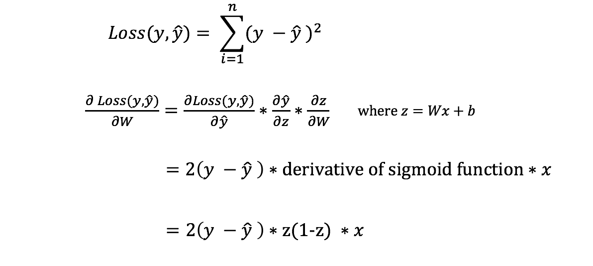
Phew! That was ugly but it allows us to get what we needed — the derivative (slope) of the loss function with respect to the weights, so that we can adjust the weights accordingly.
Now that we have that, let’s add the backpropagation function into our python code.
neural_network_backprop.py
class NeuralNetwork:
    def __init__(self, x, y):
        self.input      = x
        self.weights1   = np.random.rand(self.input.shape[1],4)
        self.weights2   = np.random.rand(4,1)
        self.y          = y
        self.output     = np.zeros(self.y.shape)

    def feedforward(self):
        self.layer1 = sigmoid(np.dot(self.input, self.weights1))
        self.output = sigmoid(np.dot(self.layer1, self.weights2))

    def backprop(self):
        # application of the chain rule to find derivative of the loss function with respect to weights2 and weights1
        d_weights2 = np.dot(self.layer1.T, (2*(self.y - self.output) * sigmoid_derivative(self.output)))
        d_weights1 = np.dot(self.input.T,  (np.dot(2*(self.y - self.output) * sigmoid_derivative(self.output), self.weights2.T) * sigmoid_derivative(self.layer1)))

        # update the weights with the derivative (slope) of the loss function
        self.weights1 += d_weights1
        self.weights2 += d_weights2
For a deeper understanding of the application of calculus and the chain rule in backpropagation, I strongly recommend this tutorial by 3Blue1Brown.
Putting it all together
Now that we have our complete python code for doing feedforward and backpropagation, let’s apply our Neural Network on an example and see how well it does.
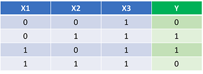
Our Neural Network should learn the ideal set of weights to represent this function. Note that it isn’t exactly trivial for us to work out the weights just by inspection alone.
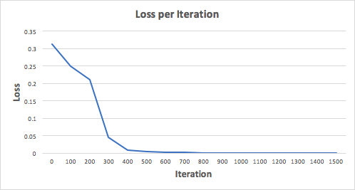
Let’s train the Neural Network for 1500 iterations and see what happens. Looking at the loss per iteration graph below, we can clearly see the loss monotonically decreasing towards a minimum. This is consistent with the gradient descent algorithm that we’ve discussed earlier.
Let’s look at the final prediction (output) from the Neural Network after 1500 iterations.
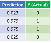
We did it! Our feedforward and backpropagation algorithm trained the Neural Network successfully and the predictions converged on the true values.
Note that there’s a slight difference between the predictions and the actual values. This is desirable, as it prevents overfitting and allows the Neural Network to generalize better to unseen data.
What’s Next?
Fortunately for us, our journey isn’t over. There’s still much to learn about Neural Networks and Deep Learning. For example:
- What other activation function can we use besides the Sigmoid function?
- Using a learning rate when training the Neural Network
- Using convolutions for image classification tasks
I’ll be writing more on these topics soon, so do follow me on Medium and keep and eye out for them!
Final Thoughts
I’ve certainly learnt a lot writing my own Neural Network from scratch.
Although Deep Learning libraries such as TensorFlow and Keras makes it easy to build deep nets without fully understanding the inner workings of a Neural Network, I find that it’s beneficial for aspiring data scientist to gain a deeper understanding of Neural Networks.
This exercise has been a great investment of my time, and I hope that it’ll be useful for you as well!
30s ad
☞ Machine Learning with Python from Scratch
☞ Deep Learning Prerequisites: Logistic Regression in Python
☞ Python Machine Learning Projects
☞ Machine Learning for Data Science
☞ Learn the essentials of Python and ArcGIS’s arcpy
☞ The Developers Guide to Python 3 Programming
Suggest:
☞ Python Machine Learning Tutorial (Data Science)
☞ Python Tutorial for Data Science
☞ Machine Learning Zero to Hero - Learn Machine Learning from scratch
☞ Complete Python Tutorial for Beginners (2019)