Automated Machine Learning on the Cloud in Python

An introduction to the future of data science, An introduction to the future of data science

An introduction to the future of data science

Two trends have recently become apparent in data science:

Data analysis and model training is done using cloud resources
Machine learning pipelines are algorithmically developed and optimized

This article will cover a brief introduction to these topics and show how to implement them, using Google Colaboratory to do automated machine learning on the cloud in Python.

Cloud Computing using Google Colab

Originally, all computing was done on a mainframe. You logged in via a terminal, and connected to a central machine where users simultaneously shared a single large computer. Then, along came microprocessors and the personal computer revolution and everyone got their own machine. Laptops and desktops work fine for routine tasks, but with the recent increase in size of datasets and computing power needed to run machine learning models, taking advantage of cloud resources is a necessity for data science.

Cloud computing in general refers to the “delivery of computing services over the Internet”. This covers a wide range of services, from databases to servers to software, but in this article we will run a simple data science workload on the cloud in the form of a Jupyter Notebook. We will use the relatively new Google Colaboratory service: online Jupyter Notebooks in Python which run on Google’s servers, can be accessed from anywhere with an internet connection, are free to use, and are shareable like any Google Doc.

Google Colab has made the process of using cloud computing a breeze. In the past, I spent dozens of hours configuring an Amazon EC2 instance so I could run a Jupyter Notebook on the cloud and had to pay by the hour! Fortunately, last year, Google announced you can now run Jupyter Notebooks on their Colab servers for up to 12 hours at a time completely free. (If that’s not enough, Google recently began letting users add a NVIDIA Tesla K80 GPU to the notebooks). The best part is these notebooks come pre-installed with most data science packages, and more can be easily added, so you don’t have to worry about the technical details of getting set up on your own machine.

To use Colab, all you need is an internet connection and a Google account. If you just want an introduction, head to colab.research.google.com and create a new notebook, or explore the tutorial Google has developed (called Hello, Colaboratory). To follow along with this article, get the notebook here. Sign into your Google account, open the notebook in Colaboratory, click File > save a copy in Drive, and you will then have your own version to edit and run.

Second, save a copy in your drive to edit

Data science is becoming increasingly accessible with the wealth of resources online, and the Colab project has significantly lowered the barrier to cloud computing. For those who have done prior work in Jupyter Notebooks, it’s a completely natural transition, and for those who haven’t, it’s a great opportunity to get started with this commonly used data science tool!

Automated Machine Learning using TPOT

Automated machine learning (abbreviated auto-ml) aims to algorithmically design and optimize a machine learning pipeline for a particular problem. In this context, the machine learning pipeline consists of:

Feature Preprocessing: imputation, scaling, and constructing new features
Feature selection: dimensionality reduction
Model Selection: evaluating many machine learning models
Hyperparameter tuning: finding the optimal model settings

There are an almost infinite number of ways these steps can be combined together, and the optimal solution will change for every problem! Designing a machine learning pipeline can be a time-consuming and frustrating process, and at the end, you will never know if the solution you developed is even close to optimal. Auto-ml can help by evaluating thousands of possible pipelines to try and find the best (or near-optimal) solution for a particular problem.

It’s important to remember that machine learning is only one part of the data science process, and automated machine learning is not meant to replace the data scientist. Instead, auto-ml is meant to free the data scientist so she can work on more valuable aspects of the process, such as gathering data or interpreting a model.

There are a number of auto-ml tools — H20, auto-sklearn, Google Cloud AutoML — and we will focus on TPOT: Tree-based Pipeline Optimization Tool developed by Randy Olson. TPOT (your “data-science assistant”) uses genetic programming to find the best machine learning pipeline.

Interlude: Genetic Programming

To use TPOT, it’s not really necessary to know the details of genetic programming, so you can skip this section. For those who are curious, at a high level, genetic programming for machine learning works as follows:

Start with an initial population of randomly generated machine learning pipelines, say 100, each of which is composed of functions for feature preprocessing, model selection, and hyperparameter tuning.
Train each of these pipelines (called an individual) and evaluate on a performance metric using cross validation. The cross validation performance represents the “fitness” of the individual. Each training run of a population is known as a generation.
After one round of training — the first generation — create a second generation of 100 individuals by reproduction, mutation, and crossover. Reproduction means keeping the same steps in the pipeline, chosen with a probability proportional to the fitness score. Mutation refers to random changes within an individual from one generation to the next. Crossover is random changes between individuals from one generation to the next. Together, these three strategies will result in 100 new pipelines, each slightly different, but with the steps that worked the best according to the fitness function more likely to be retained.
Repeat this process for a suitable number of generations, each time creating new individuals through reproduction, mutation, and crossover.
At the end of optimization, select the best-performing individual pipeline.

(For more details on genetic programming, check out this short article.)

The primary benefit of genetic programming for building machine learning models is exploration. Even a human with no time restraints will not be able to try out all combinations of preprocessing, models, and hyperparameters because of limited knowledge and imagination. Genetic programming does not display an initial bias towards any particular sequence of machine learning steps, and with each generation, new pipelines are evaluated. Furthermore, the fitness function means that the most promising areas of the search space are explored more thoroughly than poorer-performing areas.

Putting it together: Automated Machine Learning on the Cloud

With the background in place, we can now walk through using TPOT in a Google Colab notebook to automatically design a machine learning pipeline. (Follow along with the notebook here).

Our task is a supervised regression problem: given New York City energy data, we want to predict the Energy Star Score of a building. In a previous series of articles (part one, part two, part three, code on GitHub), we built a complete machine learning solution for this problem. Using manual feature engineering, dimensionality reduction, model selection, and hyperparameter tuning, we designed a Gradient Boosting Regressor model that achieved a mean absolute error of 9.06 points (on a scale from 1–100) on the test set.

The data contains several dozen continuous numeric variables (such as energy use and area of the building) and two one-hot encoded categorical variables (borough and building type) for a total of 82 features.

Raw data features

The score is the target for regression. All of the missing values have been encoded as np.nan and no feature preprocessing has been done to the data.

To get started, we first need to make sure TPOT is installed in the Google Colab environment. Most data science packages are already installed, but we can add any new ones using system commands (preceded with a ! in Jupyter):

!pip install TPOT

After reading in the data, we would normally fill in the missing values (imputation) and normalize the features to a range (scaling). However, in addition to feature engineering, model selection, and hyperparameter tuning, TPOT will automatically impute the missing values and do feature scaling! So, our next step is to create the TPOT optimizer:

tpot_regressor.py

# Import the optimizer class
from tpot import TPOTRegressor

# Create a tpot optimizer with parameters
tpot = TPOTRegressor(scoring = 'neg_mean_absolute_error', 
                     max_time_mins = 480, 
                     n_jobs = -1,
                     verbosity = 2,
                     cv = 5)

The default parameters for TPOT optimizers will evaluate 100 populations of pipelines, each with 100 generations for a total of 10,000 pipelines. Using 10-fold cross validation, this represents 100,000 training runs! Even though we are using Google’s resources, we do not have unlimited time for training. To avoid running out of time on the Colab server (we get a max of 12 hours of continuous run time), we will set a maximum of 8 hours (480 minutes) for evaluation. TPOT is designed to be run for days, but we can still get good results from a few hours of optimization.

We set the following parameters in the call to the optimizer:

scoring = neg_mean_absolute error: Our regression performance metric
max_time_minutes = 480: Limit evaluation to 8 hours
n_jobs = -1: Use all available cores on the machine
verbosity = 2: Show a limited amount of information while training
cv = 5: Use 5-fold cross validation (default is 10)

There are other parameters that control details of the genetic programming method, but leaving them at the default works well for most cases. (If you want to play around with the parameters, check out the documentation.)

The syntax for TPOT optimizers is designed to be identical to that for Scikit-Learn models so we can train the optimizer using the .fit method.

# Fit the tpot optimizer on the training data
tpot.fit(training_features, training_targets)

During training, we get some information displayed:

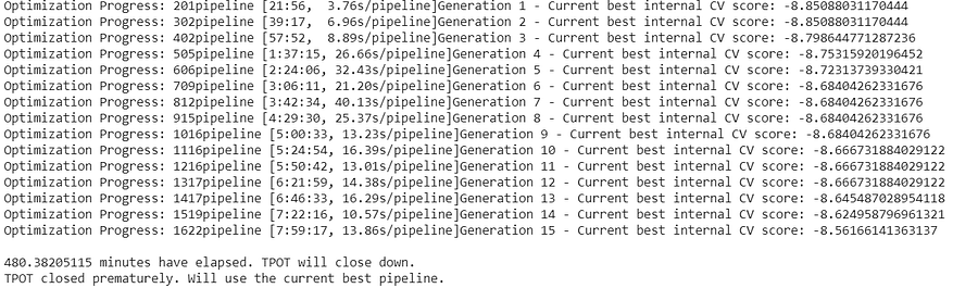
Due to the time limit, our model was only able to get through 15 generations. With 100 populations, this still represents 1500 different individual pipelines that were evaluated, quite a few more than we could have tried by hand!

Once the model has trained, we can see the optimal pipeline using tpot.fitted_pipeline_. We can also save the model to a Python script:

# Export the pipeline as a python script file
tpot.export('tpot_exported_pipeline.py')

Since we are in a Google Colab notebook, to get the pipeline onto a local machine from the server, we have to use the Google Colab library:

# Import file management
from google.colab import file
# Download the pipeline for local use
files.download('tpot_exported_pipeline.py')

We can then open the file (available here) and look at the completed pipeline:

tpot_optimized_ml_pipeline.py

# Preprocessing steps
imputer = Imputer(strategy="median")
imputer.fit(training_features)
training_features = imputer.transform(training_features)
testing_features = imputer.transform(testing_features)

# Final pipeline from TPOT
exported_pipeline = make_pipeline(
    StackingEstimator(estimator=LassoLarsCV(normalize=True)),
    GradientBoostingRegressor(alpha=0.95, learning_rate=0.1, loss="lad", 
                              max_depth=7, max_features=0.75, 
                              min_samples_leaf=3, min_samples_split=18, 
                              n_estimators=100, subsample=0.60)
)

We see that the optimizer imputed the missing values for us and built a complete model pipeline! The final estimator is a stacked model meaning that it uses two machine learning algorithms ( [LassoLarsCV](http://scikit-learn.org/stable/modules/generated/sklearn.linear_model.LassoLarsCV.html) and [GradientBoostingRegressor](http://scikit-learn.org/stable/modules/generated/sklearn.ensemble.GradientBoostingRegressor.html) ), the second of which is trained on the predictions of the first (If you run the notebook again, you may get a different model because the optimization process is stochastic). This is a complex method that I probably would not have been able to develop on my own!

Now, the moment of truth: performance on the testing set. To find the mean absolute error, we can use the .score method:

# Evaluate the final model
print(tpot.score(testing_features, testing_targets))
8.642

In the series of articles where we developed a solution manually, after many hours of development, we built a Gradient Boosting Regressor model that achieved a mean absolute error of 9.06. Automated machine learning has significantly improved on the performance with a drastic reduction in the amount of development time.

From here, we can use the optimized pipeline and try to further refine the solution, or we can move on to other important phases of the data science pipeline. If we use this as our final model, we could try and interpret the model (such as by using LIME: Local Interpretable Model-Agnostic Explainations) or write a well-documented report.

Conclusions

In this post, we got a brief introduction to both the capabilities of the cloud and automated machine learning. With only a Google account and an internet connection, we can use Google Colab to develop, run, and share machine learning or data science work loads. Using TPOT, we can automatically develop an optimized machine learning pipeline with feature preprocessing, model selection, and hyperparameter tuning. Moreover, we saw that auto-ml will not replace the data scientist, but it will allow her to spend more time on higher value parts of the workflow.

While being an early adopter does not always pay off, in this case, TPOT is mature enough to be easy to use and relatively issue-free, yet also new enough that learning it will put you ahead of the curve. With that in mind, find a machine learning problem (perhaps through Kaggle) and try to solve it! Running automatic machine learning in a notebook on Google Colab feels like the future and with such a low barrier to entry, there’s never been a better time to get started!

Learn More

☞ Interactive Data Visualization with Python & Bokeh

☞ Master the Python Interview | Real Banks&Startups questions

☞ Ensemble Machine Learning in Python: Random Forest, AdaBoost

☞ Python Network Programming - Part 1: Build 7 Python Apps

☞ Deep Learning Prerequisites: Logistic Regression in Python

Suggest:

☞ Machine Learning Zero to Hero - Learn Machine Learning from scratch

☞ Python Machine Learning Tutorial (Data Science)

☞ Platform for Complete Machine Learning Lifecycle

☞ Introduction to Machine Learning with TensorFlow.js

☞ Python Tutorial for Data Science

☞ Data Science at Shopify