Bayesian Optimization in Python with Hyperopt

A hands-on example for learning the foundations of a powerful optimization framework
Although finding the minimum of a function might seem mundane, it’s a critical problem that extends to many domains. For example, optimizing the hyperparameters of a machine learning model is just a minimization problem: it means searching for the hyperparameters with the lowest validation loss.
Bayesian optimization is a probabilistic model based approach for finding the minimum of any function that returns a real-value metric. This function may be as simple as f(x) = x², or it can be as complex as the validation error of a deep neural network with respect to hundreds of model architecture and hyperparameter choices.
Recent results suggest Bayesian hyperparameter optimization of machine learning models is more efficient than manual, random, or grid search with:
- Better overall performance on the test set
- Less time required for optimization
Clearly, a method this powerful has to be extremely hard to use right? Fortunately, there are a number of Python libraries such as Hyperopt that allow for simple applications of Bayesian optimization. In fact, we can do basic Bayesian optimization in one line!
one_line_hyperopt.py
import numpy as np
from hyperopt import hp, tpe, fmin

# Single line bayesian optimization of polynomial function
best = fmin(fn = lambda x: np.poly1d([1, -2, -28, 28, 12, -26, 100])(x),
            space = hp.normal('x', 4.9, 0.5), algo=tpe.suggest,
            max_evals = 2000)
If you can understand everything in the above code, then you can probably stop reading and start using this method. If you want a little more explanation, in this article, we’ll go through the basic structure of a Hyperopt program so later we can expand this framework to more complex problems, such as machine learning hyperparameter optimization. The code for this article is available in a Jupyter Notebook on GitHub.
Bayesian Optimization Primer
Optimization is finding the input value or set of values to an objective function that yields the lowest output value, called a “loss”. The objective function f(x) = x² has a single input and is a 1-D optimization problem. Typically, in machine learning, our objective function is many-dimensional because it takes in a set of model hyperparameters. For simple functions in low dimensions, we can find the minimum loss by trying many input values and seeing which one yields the lowest loss. We could create a grid of input values and try all of them — grid search — or randomly pick some values — random search. As long as evaluations of the objective function (“evals”) are cheap, these uninformed methods might be adequate. However, for complex objective functions like the 5-fold cross validation error of a neural network, each eval of the objective function means training the network 5 times!
For models that take days to train, we want a way to limit calls to the evaluation function. Random search is actually more efficient than grid search for problems with high dimensions, but is still an uniformed method where the search does not use previous results to pick the next input values to try. Let’s see if you’re smarter than random search. Say we have the following results from training a random forest for a regression task:
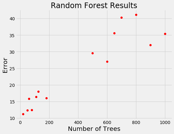
If you were picking the next number of trees to evaluate, where would you concentrate? Clearly, the best option is around 100 trees because a smaller number of trees has tended to yield a lower loss. You’ve basically just done Bayesian optimization in your head: using the previous results, you formed a probabilistic model of the objective function which said that a smaller number of trees is likely to result in a lower error.
Bayesian optimization, also called Sequential Model-Based Optimization (SMBO), implements this idea by building a probability model of the objective function that maps input values to a probability of a loss: p (loss | input values). The probability model, also called the surrogate or response surface, is easier to optimize than the actual objective function. Bayesian methods select the next values to evaluate by applying a criteria (usually Expected Improvement) to the surrogate. The concept is to limit evals of the objective function by spending more time choosing the next values to try.
Bayesian Reasoning means updating a model based on new evidence, and, with each eval, the surrogate is re-calculated to incorporate the latest information. The longer the algorithm runs, the closer the surrogate function comes to resembling the actual objective function. Bayesian Optimization methods differ in how they construct the surrogate function: common choices include Gaussian Processes, Random Forest Regression, and, the choice in Hyperopt, the Tree Parzen Estimator (TPE).
The details of these methods can be a little tough to understand (I wrote a high-level overview here), and it’s also difficult to figure out which works the best: if you read articles by the designers of the algorithms, each claim their method is superior! However, the particular algorithms does not matter as much as upgrading from random/grid search to Bayesian Optimization. Using any library (Spearmint, Hyperopt, SMAC) will be fine for getting started! With that in mind, let’s see how to put Bayesian optimization into practice.
Optimization Example in Hyperopt
Formulating an optimization problem in Hyperopt requires four parts:
- Objective Function: takes in an input and returns a loss to minimize
- Domain space: the range of input values to evaluate
- Optimization Algorithm: the method used to construct the surrogate function and choose the next values to evaluate
- Results: score, value pairs that the algorithm uses to build the model
Once we know how to specify these four parts, they can be applied to any optimization problem. For now, we will walk through a basic problem.
Objective Function
The objective function can be any function that returns a real value that we want to minimize. (If we have a value that we want to maximize, such as accuracy, then we just have our function return the negative of that metric.)
Here we will use polynomial function with the code and graph shown below:
simple_polynomial_objective.py
import numpy as np

def objective(x):
    """Objective function to minimize"""

    # Create the polynomial object
    f = np.poly1d([1, -2, -28, 28, 12, -26, 100])

    # Return the value of the polynomial
    return f(x) * 0.05
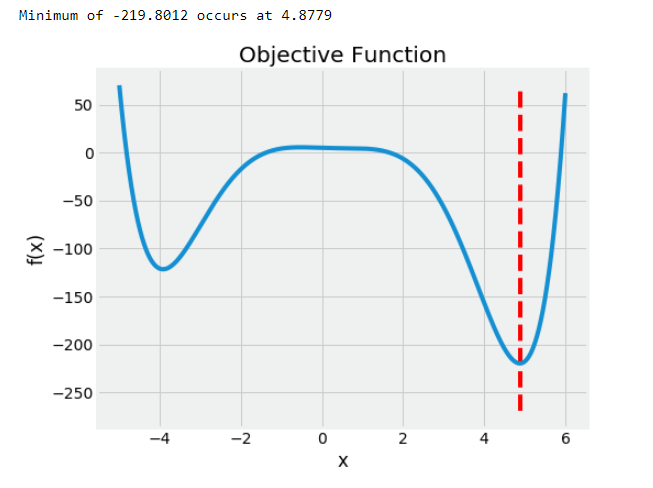
This problem is 1-D because we are optimizing over a single value, x. In Hyperopt, the objective function can take in any number of inputs but must return a single loss to minimize.
Domain Space
The domain space is the input values over which we want to search. As a first try, we can use a uniform distribution over the range that our function is defined:
from hyperopt import hp
# Create the domain space
space = hp.uniform('x', -5, 6)
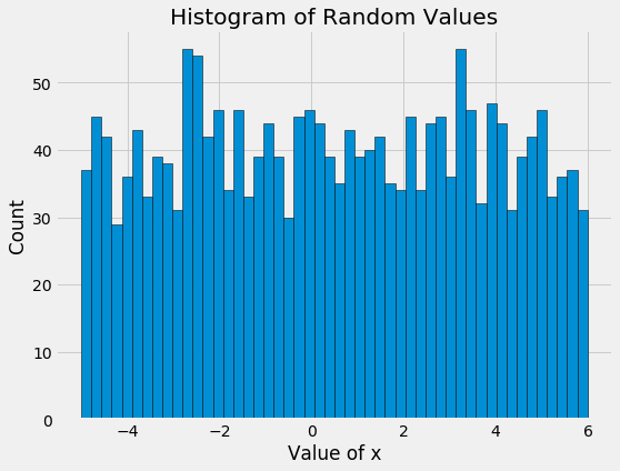
To visualize the domain, we can draw samples from the space and plot the histogram:

If we have an idea where the best values are, then we can make a smarter domain that places more probability in higher scoring regions. (See the notebook for an example of using a normal distribution on this problem.)
Optimization Algorithm
While this is technically the most difficult concept, in Hyperopt creating an optimization algorithm only requires one line. We are using the Tree-structured Parzen Estimator model, and we can have Hyperopt configure it for us using the suggest method.
from hyperopt import tpe
# Create the algorithm
tpe_algo = tpe.suggest
There’s a lot of theory going on behind the scenes we don’t have to worry about! In the notebook, we also use a random search algorithm for comparison.
Results (Trials)
This is not strictly necessary as Hyperopt keeps track of the results for the algorithm internally. However, if we want to inspect the progression of the alogorithm, we need to create a Trials object that will record the values and the scores:
from hyperopt import Trials
# Create a trials object
tpe_trials = Trials()
Optimization
Now that the problem is defined, we can minimize our objective function! To do so, we use the fmin function that takes the four parts above, as well as a maximum number of trials:
*simple_optimization.py *
from hyperopt import fmin

# Run 2000 evals with the tpe algorithm
tpe_best = fmin(fn=objective, space=space,
                algo=tpe_algo, trials=tpe_trials,
                max_evals=2000)

print(tpe_best)
{'x': 4.878208088771056}
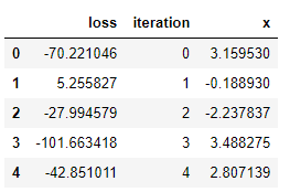
For this run, the algorithm found the best value of x (the one which minimizes the loss) in just under 1000 trials. The best object only returns the input value that minimizes the function. While this is what we are looking for, it doesn’t give us much insight into the method. To get more details, we can get the results from the trials object:
tpe_results.py
# Dataframe of results from optimization
tpe_results = pd.DataFrame({'loss': [x['loss'] for x in tpe_trials.results],
                            'iteration': tpe_trials.idxs_vals[0]['x'],
                            'x': tpe_trials.idxs_vals[1]['x']})

tpe_results.head()
Visualizations are useful for an intuitive understanding of what is occurring. For example, let’s plot the values of x evaluated in order:
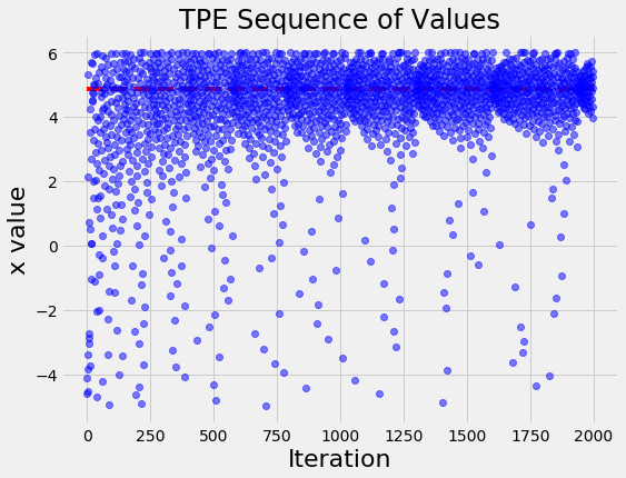
Over time, the input values cluster around the optimal indicated by the red line. This is a simple problem, so the algorithm does not have much trouble finding the best value of x.
To contrast with what a naive search looks like, if we run the same problem with random search we get the following figure:
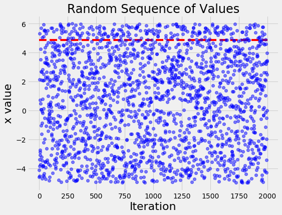
The random search basically tries values, well, at random! The differences between the values become even more apparent when we look at the histogram of values for x of the TPE algorithm and random search:
Here we see the main benefit of Bayesian model-based optimization: more concentration on promising input values. When we are searching over dozens of parameters and each eval takes hours or days, reducing the number of evals is critical. Bayesian optimization minimizes the number of evals by reasoning based on previous results what input values should be tried in the future.
(In this case, random search actually finds a value of x very close to the optimal because of the basic 1-D objective function and the number of evals.)
Next Steps
Once we have mastered how to minimize a simple function, we can extend this to any problem where we need to optimize a function that returns a real value. For example, to tune the hyperparameters of a machine learning model requires only a few adjustments to the basic framework: the objective function must take in the model hyperparameters and return the validation loss, and the domain space will need to be specific to the model.
For an idea what this looks like, I wrote a notebook where I tune the hyperparameters of a gradient boosting machine which will be the next article!
Conclusions
Bayesian model-based optimization is intuitive: choose the next input values to evaluate based on the past results to concentrate the search on more promising values. The end outcome is a reduction in the total number of search iterations compared to uninformed random or grid search methods. Although this was only a simple example, we can take the concepts here and use them in a wide variety of useful situations.
The takeaways from this article are:
- Bayesian Optimization is an efficient method for finding the minimum of a function that works by constructing a probabilistic (surrogate) model of the objective function
- The surrogate is informed by past search results and, by choosing the next values from this model, the search is concentrated on promising values
- The overall outcome of these method is reduced search time and better values
- These powerful techniques can be implemented easily in Python libraries like Hyperopt
- The Bayesian optimization framework can be extended to complex problems including hyperparameter tuning of machine learning models
Suggest:
☞ Python Machine Learning Tutorial (Data Science)
☞ Python Tutorial for Data Science
☞ Machine Learning Zero to Hero - Learn Machine Learning from scratch
☞ Learn Python in 12 Hours | Python Tutorial For Beginners